Trying to figure out the problem

[syazaaoa95]

Based on my previous question (discussion on the topic How To Split My Data….) I wanted to follow the instructions of a few suggestions given in the comment. 

but I end up, getting error. 

why? Because I don’t have the TEXTSPLIT function in my excel. 

it’s a bit difficult for me to continue on achieving my goals. :downcast_face_with_sweat:

Text to columns only can be split my sentences if there are the same delimiters or parantheses (same all the way down of all the sentences).

but due to my each data have not have consistent for me split the text, so it becames difficult to continue using the Text to Columns.

so the suggestion given from my fellow friends that comment on my questions is the function  cannot be used on my Excel. 

such as TEXTSPLIT / SPLIT 

is there any suggestion for me to move forward in a good ideas?

[#2 · Accepted solution]

@syazaaoa95 

=LEFT(A3,MIN(IFERROR(SEARCH("IR",A3),9^99),IFERROR(SEARCH("CS",A3),9^99),IFERROR(SEARCH("I5",A3),9^99))-2)

=RIGHT(A3,LEN(A3)-(MIN(IFERROR(SEARCH("IR",A3),9^99),IFERROR(SEARCH("CS",A3),9^99),IFERROR(SEARCH("I5",A3),9^99))-2)-1)

You can try these formulas. The first formula is in cell B3 and filled across range B3:B5 and the second formula is in cell B7 and filled across range B7:B9. Both formulas check which delimiter occurs first in a string. Then this is used to split the text into two results.  

[#3]

Hi Pawn.

Thank you so much for the response.

Meaning that, if I were to use the split on my overall data, meaning that I had to enter min(iferror(search(" ") for each of the different delimiter? If it had any different?

[#4]

@syazaaoa95 

You are welcome. For every additional delimiter you can add an IFERROR(SEARCH(   to the MIN function. I've highlighted the added part in the formula below.

=LEFT(A3,MIN(IFERROR(SEARCH("IR",A3),9^99),IFERROR(SEARCH("CS",A3),9^99),IFERROR(SEARCH("I5",A3),9^99),IFERROR(SEARCH("ABC",A3),9^99))-2)

[#5]

Thank you so much Pawn. It does help me a lot!!!

if I got any question, can I just directly ask you? or is it okay for you?

[#6]

@OliverScheurich 

Hi Pawn,

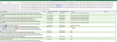
Look. I've tried for another data.
It seems like it have case sensitive. which it reaches the letters from the left first. Because my data have Original "AL" which it reads from my Search("AL", formula.

How to solve this :(

[#7]

@syazaaoa95 

And also about this?

How to do. I'm sorry for asking

[#8]

@syazaaoa95 

I should have used FIND instead of SEARCH in order to perform an exact match including small or capital letters.

This is the formula in cell B3:

=LEFT(A3,MIN(IFERROR(FIND("IR",A3),9^99),IFERROR(FIND("CS",A3),9^99),IFERROR(FIND("I5",A3),9^99),IFERROR(FIND("ABC",A3),9^99),IFERROR(FIND("AL",A3),9^99),IFERROR(FIND("SF",A3),9^99))-2)

This is the formula in cell C3:

=RIGHT(A3,LEN(A3)-(MIN(IFERROR(FIND("IR",A3),9^99),IFERROR(FIND("CS",A3),9^99),IFERROR(FIND("I5",A3),9^99),IFERROR(FIND("ABC",A3),9^99),IFERROR(FIND("AL",A3),9^99),IFERROR(FIND("SF",A3),9^99))-2)-1)

[#9]

@OliverScheurich 

Thank you so much for bearing with me. 

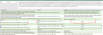
Now I have my problem with the zero value.

I'm trying to add up with IFERROR(SEARCH(" ",BLANK)
I want to return the output to be blank, so that which of the description that does not have model, it will be return in blank. 

so that it won't return #value.

thank you Pawn and sorry for asking too much !

[#10]

@syazaaoa95 

Do you want a blank cell if none of the values is found in a cell? For example if none of these values {"IR"."CS"."I5"."ABC"."AL"."SF"} is found in cell A3.

=IFERROR(LEFT(A3,IF(SUMPRODUCT(N(ISNUMBER(FIND(({"IR","CS","I5","ABC","AL","SF"}),A3))))=0,"",MIN(IFERROR(FIND("IR",A3),9^99),IFERROR(FIND("CS",A3),9^99),IFERROR(FIND("I5",A3),9^99),IFERROR(FIND("ABC",A3),9^99),IFERROR(FIND("AL",A3),9^99),IFERROR(FIND("SF",A3),9^99))-2)),"")

=IF(B3="","",RIGHT(A3,LEN(A3)-(MIN(IFERROR(FIND("IR",A3),9^99),IFERROR(FIND("CS",A3),9^99),IFERROR(FIND("I5",A3),9^99),IFERROR(FIND("ABC",A3),9^99),IFERROR(FIND("AL",A3),9^99),IFERROR(FIND("SF",A3),9^99))-2)-1))

Maybe these formulas return the intended result.

[#11]

@syazaaoa95 

I saw your screenshot after i had already answered. I think this can be solved by wrapping the formula into IFERROR. I've highlighted the IFERROR in the sample formula.

=IFERROR(RIGHT(A3,LEN(A3)-(MIN(IFERROR(FIND("IR",A3),9^99),IFERROR(FIND("CS",A3),9^99),IFERROR(FIND("I5",A3),9^99),IFERROR(FIND("ABC",A3),9^99),IFERROR(FIND("AL",A3),9^99),IFERROR(FIND("SF",A3),9^99))-2)-1),"")