The visualization of the numbers in excel is not "correct"

[danielaanchico]

Hello! I hope everyone is great. I'm here with the hope of solving my problem.

I have to do an assignment for uni, and we have to work with a database from the DANE, a departmet of stadistics about my country, Colombia. Here is the link:  https://microdatos.dane.gov.co/index.php/catalog/708/get-microdata

We need to use the ones called "Hogares" and "Personas". The problem comes when I have to work with the colum "lp", or "ingtot", among others  and do some PivotTable. 

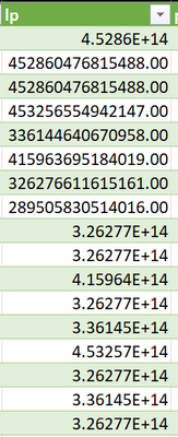
As you can see in the image, the numbers are very long, but Excel is not making them "smaller". It's a big deal cause, when I'm doing the average, the numbers still like that, and it's not possible to do the correct analysis of people being poor or not. For example, someone that won 2.3 billion pesos, appear that is poor, because the number was less than the poverty line. 

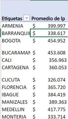
This database is the same for every of my partners, but for them, the numbers are right, as you can see here: 

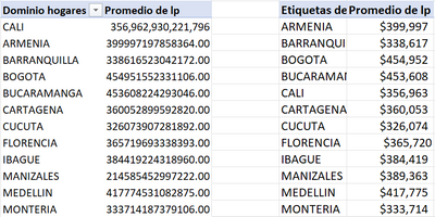
A comparison between my pivot table and the one of my partners:

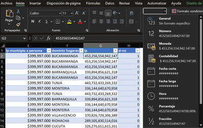
Although in the formula bar, the numbers appear complete, in the pivotTable, the numbers show like this, and it's in this form that I need them to be, so I can continue doing my job. I have already tried to change the system separators, but it hasn't work. And yes, I have tried to change the format of the cells many times too.

If anyone could help, I would be really grateful

[#2]

@danielaanchico 

To resolve this issue, you can may be try changing your regional settings in Windows.

Here's how:

1. Click on the Start menu and type "Region" in the search box.
2. Click on "Region settings" to open the Region settings window.
3. Under the "Formats" tab, make sure the "Format" drop-down menu is set to "Spanish (Colombia)".
4. Under the "Additional settings" section, click on the "Numbers" tab.
5. In the "Decimal symbol" field, enter a comma (",").
6. In the "Digit grouping symbol" field, enter a period (".").
7. Click "Apply" and then "OK" to save the changes.

After changing these settings, try refreshing your PivotTable to see if the numbers display correctly. If the issue persists, try changing the format of the cells in the PivotTable to "Number" or "Currency" and adjust the decimal places as needed.

I hope this helps!

[#3]

@NikolinoDE 

Hello there! Thank you for your answer, I really appreciate it, but unfortunately it didn't work :( The advanced settings in my computer are already like you said. I changed the format of my cells and refreshed the pivot table, but the problem still the same there and in my cells of the column from the database:

[#4]

@danielaanchico 

In that case, there are a few other things you can try:

1. Check if the numbers are being imported into Excel as text. You can check this by selecting the cells with the numbers, right-clicking, and selecting "Format Cells". In the Format Cells dialog box, select the "General" category and click "OK". If the numbers change to the correct format, then they were being imported as text and you can try importing them again as numbers.
2. Use the VALUE function to convert the text-formatted numbers to actual numbers. To do this, insert a new column next to the column with the text-formatted numbers, enter the formula "=VALUE(cell)" in the first cell of the new column (replace "cell" with the reference to the corresponding cell in the original column), and then drag the formula down to apply it to all the cells in the new column. Then, use the new column for your pivot table.
3. Use Power Query to import the data and transform it before creating the pivot table. Power Query is a tool in Excel that allows you to import, transform, and clean data from various sources. You can use Power Query to convert the text-formatted numbers to actual numbers before creating the pivot table.

Here's how to do it:

• Click the "Data" tab and select "From Other Sources" -> "From Microsoft Query".
• In the "Choose Data Source" dialog box, select "Excel Files" and click "OK".
• In the "Connect" dialog box, select the Excel file containing the data and click "OK".
• In the "Query Wizard - Choose Columns" dialog box, select the columns you want to import and click "Next".
• In the "Query Wizard - Filter Data" dialog box, you can apply any filters you need and click "Next".
• In the "Query Wizard - Sort Order" dialog box, you can specify the sort order of the data and click "Next".
• In the "Query Wizard - Finish" dialog box, select "View data or edit query in Microsoft Query" and click "Finish".
• In Microsoft Query, select the column with the text-formatted numbers and click "Format" -> "Number".
• In the "Number" dialog box, select the desired format for the numbers and click "OK".
• Click "File" -> "Return Data to Microsoft Excel".
• In the "Import Data" dialog box, select where you want to place the data and click "OK".
• The imported data will now be in a table in Excel, which you can use to create your pivot table.

I'm at my and AI’s wit's end with this, hope it helps :).