Summing values based on Condition

[CHende77]

Hello Excel Experts,

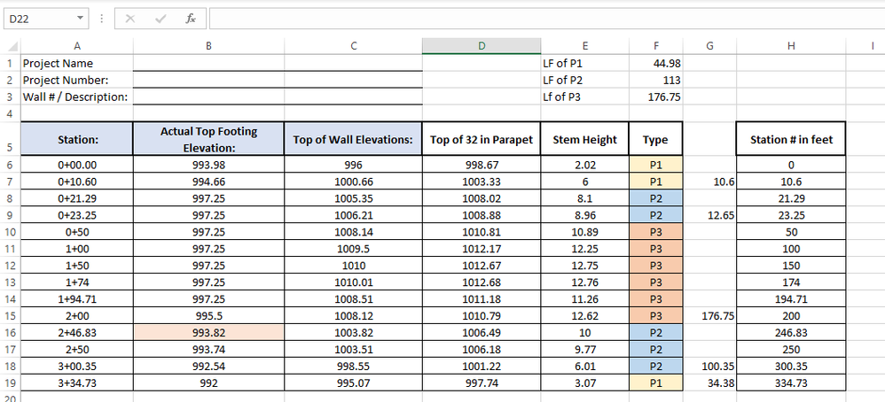
I am using excel (version 2206) on a PC with Windows 10. I want to be able to determine lengths of walls based on their type (P1, P2, or P3). The sheet I have will give the type and the station numbers in feet. I'd like to have some way (formula or VBA is fine) that column G could end up as shown. I've done it manually here, by subtracting values from Column H. I'd like the solution to be applicable to any wall in the future, where columns F and H will be completely different. Normally, the type would not be colored, so please avoid any solution with conditional formatting.

I'd also like to have the total length for each type of wall posted up above in cells F1:F3, if possible.

 Thanks in advance!

[#2 · Accepted solution]

@CHende77 

Hi,
based on the example you provided you could try to replicate your result by using this formula:
Formula for cell G6:
=IF($F6<>$F7;IF($F6<>$F7;$H6;0)-IF(ISNUMBER($G5);SUM($G$5:$G5);0);0)
Then copy & paste the formula down to the last row of your table.
Now this should work, if you don't change the layout of the sheet.

To return the sum for each type you could try this:
Formula for cell F1 (copy & paste to cell F2 and cell F3):
=SUMIF($F$6:$F$19;MID($E1;FIND("P";$E1;1);LEN($E1)-6);$G$6:$G$19)
Now here you need to reshape the cell ranges (underlined in the formula above) based on the range of your table. For example if your table ranges from row 6 to row 25 you would exchange all 19's in the formula with a 25.

Hope it helps.

[#3]

Thanks a bunch, very nice solution!