Summing positive/negative amounts across sheets

[BillF44]

Message Edited.  Sorry for my mistakes in the original.

----------------------------------------------------------------

Sum Profit and/or Loss from a column from 1 sheet (Raw) in 2nd sheet (Stats), for a set number of rows. 

Data sheet 1 (Raw):

100 rows of pos./neg. amounts in a column in sheet 1(Raw).  Want formula to find total pos./neg. amts. in the last 10 rows (This number is variable by the user, could be any pos. number from 1 to infinity).  Ex:  last 10 rows contain 7 rows with pos. amts. and 3 rows containing neg. amts.  Two formulas, Case 1:one summing pos. amts. and Case 2:one summing neg. amts.

Case 1:

1  $1.00

2  $0.23

3  -$3.32

4  $22.65

5  -$2.10

6  $78.44

7  $19.46

8  $19.72

9  $1974

10  -$16.45

11  $22.20

12  -$100.75

Results on the Stats Sheet should be Positive Amount = $161.24 and Negative Amount = -$21.87.

Case 2: On second sheet, find Pos. and Neg. amounts for the last 3 Positive Amounts and for the last 3 Negative Amounts.

Results:  Last(Most recent- Rows 1, 2, 3) 3 Positive Amounts = $23.88.  Last(Most recent 2, 5, 10) 3 Negative Amounts = -$21.87.

I have struggled with these two calculations for quite so time and would really be so GRATEFUL for some solution.

Thanks

[#2]

@BillF44 

It depends on which Excel version / platform you are. As variant

=SUMPRODUCT( data * ( SIGN(data) > 0) )
=SUMPRODUCT( data * ( SIGN(data) < 0) )
=SUM( INDEX( data, AGGREGATE(14, 6, 1/(data>0)*ROW(data), {1,2,3} ) ) )
=SUM( INDEX( data, AGGREGATE(14, 6, 1/(data<0)*ROW(data), {1,2,3} ) ) )

assuming data is from first row, otherwise to adjust a bit.

[#3]

Thank you very much Sergei.
I entered the following into my 2nd sheet (Stats).

=SUMPRODUCT('Funded Bootcamp.xlsm'!Profit.S:Profit.E * (+('Funded Bootcamp.xlsm'!Profit.S:Profit.E)>0)) =SUMPRODUCT('Funded Bootcamp.xlsm'!Profit.S:Profit.E * (+('Funded Bootcamp.xlsm'!Profit.S:Profit.E) < 0)) =SUM(INDEX('Funded Bootcamp.xlsm'!Profit.S:Profit.E,AGGREGATE(14, 6, 1/('Funded Bootcamp.xlsm'!Profit.S:Profit.E>0)*ROW('Funded Bootcamp.xlsm'!Profit.S:Profit.E), {1,2,3}))) =SUM(INDEX('Funded Bootcamp.xlsm'!Profit.S:Profit.E,AGGREGATE(14, 6, 1/('Funded Bootcamp.xlsm'!Profit.S:Profit.E < 0) * ROW('Funded Bootcamp.xlsm'!Profit.S:Profit.E), {1,2,3})))

Am getting result = FALSE. I do not see a typing error, but maybe you will.
My Spread Sheet name is "Funded Bootcamp.xlsm" and my two sheets are "Orders" and "STATS_1". The Profit column is Column "W" and I have Defined Names in cell "W2" and at this point in cell "W10856", quite a bit of data here.

Hope this additional info plus corrections to original posting clarifies my needs somewhat.

[#4]

@BillF44 

Sorry, I didn't catch. If Profit is the name of the column, e.g. =Orders!$W:$W, what is Profit.S, etc. ?

[#5]

@Sergei Baklan 

Good Morning Sergei.
Profit.S is Defined Name for the start of Profit column. i.e. Column W, row 2, or $W$2 in my sheet "Orders". Profit.E is highest row in same column. It increases as I insert new rows into the "Orders" sheet using "Insert copied cells", currently, in my up to date spreadsheet it is W10855.  Row 1 is most recent data and row 10855 is oldest data.  Just an FYI, this spreadsheet is a record of my FOREX Trading going back to October 2021.  Hope that I am making sense to you, please tell me if I need to explain more or better.

[#6]

@BillF44 

If in first file we have

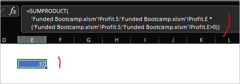
when in another file

formula

=SUMPRODUCT(
   'Funded Bootcamp.xlsm'!Profit.S:'Funded Bootcamp.xlsm'!Profit.E *
   ('Funded Bootcamp.xlsm'!Profit.S:'Funded Bootcamp.xlsm'!Profit.E>0))

works. Perhaps the same for other formulae.