SUMIF on Mortgage Amortization Sheet

[Robert_Jeter]

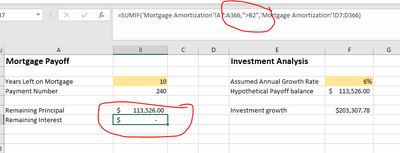
I'm using a SUMIF formula to determine the remaining amount of interest on another sheet based on the number payment remaining on a mortgage. In the criteria, if I use a specific number, say payment "12", it calculates correctly. If I use a reference to a cell which would indicate the payment number, say "B2", it does not calculate. Any idea on how to make this criteria work? Thanks.

[#2]

@Robert_Jeter 

Can you show us the actual formulas, the one that does work and the one that doesn't? It probably has to do with some minor aspect of how you've written it. 

And if you could describe more fully (or add a picture of) the spreadsheet that contains the data the formula is referring to, that could help as well.

[#3]

@mathetes Sure. I've attached a few. The first is the actual mortgage amortization sheet. Calculates as it should. The second two are the specific formula I'm using SUMIF for to calculate the total amount of interest remaining to be paid. If I use the specific payment number, it calculates the total amount of interest. If I use a reference to the cell, it does not.

[#4]

@Robert_Jeter 

One of the reasons I enjoy answering questions here at the Excel techcommunity site is that I frequently learn something I didn't know. This is one of those cases.

Turns out that the syntax for SUMIF, when you're referencing the content of a cell, just isn't quite as straightforward as you might expect. Here's what I discovered:

A value from another cell can be included in criteria using concatenation. In the example below, SUMIF will return the sum of all sales over the value in G4.  Notice the greater than operator (>), which is text, must be enclosed in quotes. The formula in G5 is:

=SUMIF(D5:D9,">"&G4) // sum if greater than G4

The full page from which I got that reference is https://exceljet.net/excel-functions/excel-sumif-function

So your formula should end up reading thus:

=SUMIF('Mortgage Amortization'!A7:A366,">"&B3,'Mortgage Amortization'!D7:D366)

[#5]

@mathetes 

I'm trying to take it up a notch. I have the exact same amortization schedule as Rob. However, 

I'm not trying to output a summation of the 30 years but rather a summation of a column based on a dynamic date (i.e. one sum per year over 30-years).

The date range will be dynamic but how do I loop this into the summation formula??

- Basically if the mortgage starts in May 2023 then I'd like to do a summation of my interest and principal columns up until December 2023 (i.e. the first year).

- Then I would like to do a straightforward calculation January to December (for the next 28 years, i.e. 2024 to 2052).

- The last year's calculation would be dynamic once again as it will only be from January to April only (the 30th year i.e. 2053)

Do you happen to know how I could possibly do this in Excel. The loan start date is a manual input at the beginning of the sheet (i.e. May 2023) 

[#6]

@RJ123185 I'm not sure I understand exactly but I think what you want is to use SUMIFS (i.e. plural form).  It is important to note that the format of the SUMIFS() is different than the SUMIF() because you must have the sum column and it is the first argument instead of the optional last.  So in the above example you could do something like:

=SUMIF('Mortgage Amortization'!D7:D366,'Mortgage Amortization'!A7:A366,">"&B3,'Mortgage Amortization'!A7:A366,"<="&B4)

where col D has what is to be summed, col A are the dates and then B3 and B4 are the start and end dates of the desired range.

I hope that helps get you in the right direction.