- Home
- Microsoft 365
- Excel
- Re: SumIF (2 criteria & currency conversion)
SumIF (2 criteria & currency conversion)
- Subscribe to RSS Feed
- Mark Discussion as New
- Mark Discussion as Read
- Pin this Discussion for Current User
- Bookmark
- Subscribe
- Printer Friendly Page
- Mark as New
- Bookmark
- Subscribe
- Mute
- Subscribe to RSS Feed
- Permalink
- Report Inappropriate Content
Apr 21 2023 07:38 AM
Hello experts,
Please see attached example file.
I need to sum an [Amount] if the [Type] column = *Liquid* but only if the [Paid Date] is null. But I also need to convert the [Amount] if the currency is either EUR or DKK. If EUR then multiply by 1.1 and if DKK then divide by 6.7.
thank you very much. Let me know if not clear.
- Labels:
-
Excel
-
Formulas and Functions
- Mark as New
- Bookmark
- Subscribe
- Mute
- Subscribe to RSS Feed
- Permalink
- Report Inappropriate Content
Apr 21 2023 07:59 AM
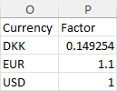
SolutionI'd create a lookup range. In the attached workbook it is in O2:P4 but it can be anywhere, even on another sheet.
(P2 contains the formula =1/6.7)
You can then use the formula
=SUMPRODUCT(C2:C5,XLOOKUP(B2:B5,O2:O4,P2:P4),(D2:D5="Liquid")*(E2:E5=""))
If you don't have Microsoft 365 or Office 2021:
=SUMPRODUCT(C2:C5,VLOOKUP(B2:B5,O2:P4,2,FALSE),(D2:D5="Liquid")*(E2:E5=""))
- Mark as New
- Bookmark
- Subscribe
- Mute
- Subscribe to RSS Feed
- Permalink
- Report Inappropriate Content
Apr 21 2023 09:25 AM
My variant:
=LET(
    dkk, SUMIFS(amt, curr, "DKK", type, "Liquid", paid, "") / 6.7,
    eur, SUMIFS(amt, curr, "EUR", type, "Liquid", paid, "") * 1.1,
    dkk + eur
)
- Mark as New
- Bookmark
- Subscribe
- Mute
- Subscribe to RSS Feed
- Permalink
- Report Inappropriate Content
Apr 21 2023 03:59 PM
- Mark as New
- Bookmark
- Subscribe
- Mute
- Subscribe to RSS Feed
- Permalink
- Report Inappropriate Content
Apr 22 2023 01:50 AM
Just pick one - it doesn't matter which one.
- Mark as New
- Bookmark
- Subscribe
- Mute
- Subscribe to RSS Feed
- Permalink
- Report Inappropriate Content
Apr 22 2023 12:31 PM
Just to reinforce the fact that there is usually a choice of solution approach
= LET(
    factoredAmt, amount * XLOOKUP(Curr, Currency, Factor),
    criterion,   (type="Liquid") * (paid_date=""),
    filteredAmt, FILTER(factoredAmt, criterion),
    SUM(filteredAmt)
  )
(For 'best' go with the one you use or, failing that, settle for the first correct solution)
- Mark as New
- Bookmark
- Subscribe
- Mute
- Subscribe to RSS Feed
- Permalink
- Report Inappropriate Content
Apr 23 2023 06:20 AM
Accepted Solutions
- Mark as New
- Bookmark
- Subscribe
- Mute
- Subscribe to RSS Feed
- Permalink
- Report Inappropriate Content
Apr 21 2023 07:59 AM
SolutionI'd create a lookup range. In the attached workbook it is in O2:P4 but it can be anywhere, even on another sheet.
(P2 contains the formula =1/6.7)
You can then use the formula
=SUMPRODUCT(C2:C5,XLOOKUP(B2:B5,O2:O4,P2:P4),(D2:D5="Liquid")*(E2:E5=""))
If you don't have Microsoft 365 or Office 2021:
=SUMPRODUCT(C2:C5,VLOOKUP(B2:B5,O2:P4,2,FALSE),(D2:D5="Liquid")*(E2:E5=""))
