Sum shown in colour to be higher or lower than a target number

[gnasher]

Hi,

If I have cell 3 showing the result of a deduction of a number in cell 2 from a number in cell 1, is there a way for cell 3 to be instructed to give this result but turn either the text of the number or the cell itself to the colour red if the value is higher than a value of say"10" referenced as a target number to reach in another cell 4.

Conversely, if the value is lower than "10" in cell 4, cell 3 would be instructed to show this lower number result but either the text or the cell will turn to the colour green.

Thanks in advance for your help.

[#2 · Accepted solution]

@gnasher That can be done with Conditional Formatting as shown in the picture.

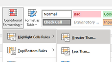
I selected cells C3:C7. Then on the Home ribbon, choose Conditional Formatting. 

Highlight Cells, greater than.....

and then enter 10 and set the format to your liking.

[#3]

@Riny_van_Eekelen 

Thanks Riny, I used your advice and by using the "greater than equal" function was able to highlight when the target was not achieved.

Pushing a little further with your advice I noticed that it does not seem to be possible to apply two simultaneous rules to the same cell though ("greater than and equal" and "less than and equal"). Do you know if it is possible to do this?

[#4]

@gnasher Yes you can. If a value has to be both >= AND <=, that would be a "between" rule. Otherwise you need to use a formula to set the rule with, for example the AND function. There are many possibilities with Conditional Formatting. Google for it and you'll find numerous examples.

[#5]

Thanks Riny, thats great advice and useful to know. So far I had been stuck on single instructions in a cell.