SUM part of SEQUENCE spill range

[Nairn1150]

Hi all, I am creating a spreadsheet to track my clock-in and clock-out times per month. As part of this, I would like to be able to sum the amount of time worked per day within a given week. The set-up for this is a Sequence function which creates the correct number of dates for the month (So I can copy the sheet and change the month, and everything updates automatically), a column to display each day's name using the spill operator ( =TEXT(A2#,"dddd") ), with the clock-in/-out times then manually entered on the right. The final column is the resultant time worked for the day.

To prevent me manually setting up the ranges of the weeks in every new month, I am trying to create a dynamic formula to sum the working times between any Sunday in the sequence, and the previous 6 days (and thus limit the sum to just each Monday-Sunday week). I am essentially looking for: If day of week is a Sunday, sum that, plus six more cells above.

My problem is stemming from the use of the spill function, as when I use the following formulae (and the many many variations I have tried) I am getting strange calculations, like summing the whole range, rather than just a portion of it, #REF errors, etc.

=IF(WEEKDAY(A2#,2)=7,SUM(OFFSET(A2#,0,2,-6)),"")

Or

=IF(WEEKDAY(A2#,2)=7,IF(DAY(A2#)>6,SUM(OFFSET(A2#,0,-6)),"Sunday before 7th"),"")

 In the second formula I am accounting for that fact that if a Sunday lands on the 1st-6th there won't be the correct number of cells above to use the standard Offset value, but I haven't figured that part out yet either.

I can use a normal Sum (by selecting cells manually) to get the correct results, I can combine the Sum function with Offset to get a range, but when combined with the spill operator (A2#) everything seems to break. Does anyone have any insights on this? Is there some way to limit the sum range while referencing a spilled cell? Is there another method I could use? (I thought something with INDIRECT maybe, but I'm not sure how I could implement that since ADDRESS doesn't work with the A2# range)

Thanks!

P.S happy to post an example file, but I can't see a way to attach a file at the moment.

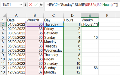
[#2 · Accepted solution]

@Nairn1150 Easiest would be to insert a column with the ISO-week number, using =ISOWEENUM(A2#). Then, you could do something like this:

File attached.

[#3]

@Riny_van_Eekelen 

Thank you for the quick reply, I like this a lot, it's very clean compared to what I was trying to do!

I initially had the same problem when using your formula. For a while I couldn't understand what I was doing wrong when implementing your approach, but I realized that it was still trying to use a spill reference (#) for the If(Cell#="Sunday"... Once I changed it to If(Cell="Sunday"... and filled that down the column everything worked as expected.

Out of curiosity I adapted my original formulas to the same style, and ditched the spill references. 

=IF(WEEKDAY(A2,2)=7,IF(DAY(A2)<7,SUM(OFFSET(A2,0,3,-DAY(A2))),SUM(OFFSET(A2,0,3,-7))),"")

This formula worked as intended, and I was able to use not just the SUM(OFFSET), but also dynamically adjust the size of the offset for split weeks by using the DAY function to set the offset range. I can't believe how close I have been skirting around this solution, and the only part letting me down was the spill range!

I wonder if my original effort is just not an intended use-case for the spill operator? I could certainly think of other uses for summing part of a spilled range, but perhaps it would require the use of helper columns, alternate functions or sum conditions etc.

In any case, thank you very much for your assistance.

[#4]

In case anyone stumbles across this thread in the future and is still looking to use the spill operator functionality, I had a little play about with the suggestion by @Riny_van_Eekelen, and I realised that the following formula works in the case of using a helper column (B) with =ISOWEEKNUM(A2#), and named range (can be substituted for regular cell references):

=IF(WEEKDAY(A2#,2)=7,SUMIF(B2#,B2#,Hours),"")

And you even add the offset back in from my original post so everything is dynamic based around the first column:

=IF(WEEKDAY(A2#,2)=7,SUMIF(B2#,B2#,OFFSET(A2#,0,3)),"")