Sum of Amount of salesperson brandwise and non brand wise

[ishaqib]

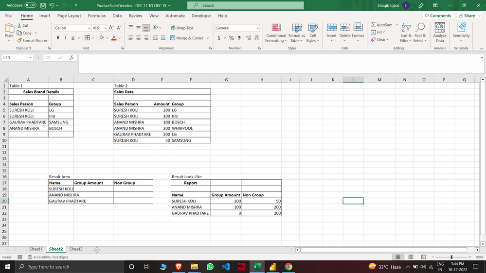
Hello Excel Family, I am trying to solve this question from last 2 hours and didn't get the accurate answer, i tried using sumproduct, sumifs, vlookup but didn't get the desired answer, Please help to get gid out of this.. 

Table 1 Contains Details of Sales Person Brand
Table 2 Contain Sales Data
Result Look like table is the final table I want..
...
Question is Suresh Koli is of LG & IFB group brand so when we sum the total amount of suresh koli sales it should sum only their brand amount i.e 200 for LG 100 For 100 Total 300 while suresh kohi sold only 50 of samsung brand so that amount will go to Non Group Column
....
One sales Person can have either one brand or multiple brand.

[#2 · Accepted solution]

@ishaqib 

=IFNA(IF(MATCH(D5&F5,$A$5:$A$8&$B$5:$B$8,FALSE),1),0)

A possible solution could be with a helper formula in cell G5. Enter the formula with ctrl+shift+enter if you don't work with Office 365 or Excel 2021. Then fill the formula down.

In cell G20:

=SUMPRODUCT((F20=$D$5:$D$10)*$E$5:$E$10*$G$5:$G$10)

In cell H20:

=SUMPRODUCT((F20=$D$5:$D$10)*$E$5:$E$10*NOT($G$5:$G$10))

[#3]

@ishaqib 

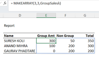
A solution that works only with Excel 365

= LET(
    p,       INDEX(person,n),
    groups,  FILTER(BrandTbl[Group],  BrandTbl[SalesPerson] = p),
    totals,  SUMIFS(SalesTbl[Amount], SalesTbl[Person],  p),
    amounts, SUMIFS(SalesTbl[Amount], SalesTbl[Person],  p, SalesTbl[Group], groups),
    Choose(option, SUM(amounts), totals - SUM(amounts), totals)
  )

[#4]

Thanks a ton for your reply sir

[#5]

Thanks a lottt sir for your reply, I got my answer