Sum cells with specific background color with filters?

[edd21475]

I came across an issue and couldn't find a proper solution on the internet, so if anyone could help, it would be greatly appreciated!

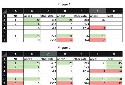
I have this type of data I'm working with at school (see Figure 1), I need to count the sum of price values in columns B D F in each row separately, but only those that have a background color of either green or red (there is only one color in each row, there is no red and green in the same row). Basically, G2 has to be the sum of B2 D2 F2 with a filter that sums only green/red cells; if it's green, fill the solution with green color as well; if red - with red; if there is no color - leave it blank. Then I will just drag it down to apply the same settings for the other rows. So the result should look like in Figure 2 G column. Afterward, the № of the row has to be filled with the same color as the respective solution in the G column. In my case A2 A3 A6 is filled with green and A4 A7 in red; if no color - don't fill with any color.

I hope I explained it well enough. Thanks in advance!

Excel version: 16.55 Excel for Mac

MacOS Catalina 10.15.7

[#2 · Accepted solution]

@edd21475 

Is this what you are looking for?

Color in range B2:F7 has to be entered manually and color in range A2:A7 is done by conditional formatting.

[#3]

Yes, this is pretty much what i need, thank you so much!

[#4]

@edd21475 

Glad it helped. I just noticed that you want to conditionally format both columns A and G. See attached file sheet "Tabelle2".

[#5]

@OliverScheurich 

I have figured out the condition formating, thank you for the reply! However, i got one more questing, maybe you could help? 

In the example you provided, the VBA doesnt update the color index if i change the color of the respective cell, i have to manually reapply the formula so the color index changes. Is there a way to make it update automatically once i change the color of the cell?

Eg.: If i change B2 to green, the index in B9 doesnt update, i will have to refresh it manually. So what i would like is once i change B2 to green, B9 automatically refreshes from 3 to 50

Looking forward to your reply!

[#6]

@edd21475 

When i open the spreadsheet i have to allow macros and then i can select for example cell C4 which has green color (in sheet Tabelle2). Then i copy the format of cell C4 and paste this format in cell B2. After this cell B9 automatically updates to 50 and cells A2 and G2 automatically are formatted in green color.