Stuck with Conditional Formatting

[CosTech1955]

I've searched high and low and not getting anywhere I need. It's probably so simple but I just can't get it to work.

I've got a training matrix document. 

I need a column to adjust the color based on upcoming expiry dates for tests taken.

Scenario:

Column A has a list of names of people to take these tests.

Column B Row 1 has a title header and then from Row 2 onwards a list of dates a test was taken. These all expire within 2 years.

Column C Row 1 has a title header and then from Row 2 onwards a list of dates another test was taken. These all expire within 3 years.

For example, if we use today's date 26/11/2022

Name	Test A (2 years expiry)	Test B (3 years expiry)
John Smith	26/11/2022 (Green)	26/11/2022 (Green)
Alex Jones	( No Entry Blank)	26/12/2019 (Orange)
Katie Jones	26/12/2020 (Orange)	26/10/2019 (Red)

I need to set the formatting so that:

No entry into the column - Blank Cell

The date entered is current and within the parameter of 2 years or 3 years from Date entered = Green

The date entered is nearing 30 days of expiry from the date entered = Orange

The date entered is expired from the date entered = Red

[#2]

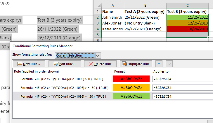
@CosTech1955 My date settings are different, but the logic is the same.

It seems you will need two sets of conditional formats; here is one set:

In text form, those formulas are:

=IF( (C2<>"")*(TODAY()-(C2+1095) > 0 ), TRUE )
=IF( (C2<>"")*(TODAY()-(C2+1095) >= -30 ), TRUE )
=IF( (C2<>"")*(TODAY()-(C2+1095) < -30 ), TRUE )

Obviously, the other set of formulas would use 730 for two years.

I presume you do not require precision that includes leap days within those two or three years.

[#3]

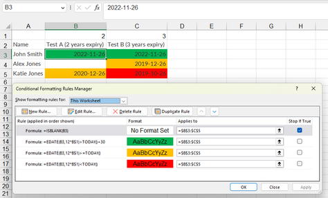
@CosTech1955 As a variant and a bit easier, I think. Note I introduced the number of years before expiry into separate cells (B1 and B2) to make it more dynamic.

File attached.

[#4]

@CosTech1955 

Select the cells in column B, starting with B2.

On the Home tab of the ribbon, select Conditional Formatting > New Rule...

Select 'Format only cells that contain'.

Leave the first drop down set to 'Cell Value'.

Select 'greater than' from the second drop down,

Enter 0 in the box next to it.

Click Format...

Activate the Fill tab.

Select red.

Click OK, then click OK again.

Repeat these steps, but instead of 0, enter the formula =EDATE(TODAY(),-24) in the box, and select orange as fill color.

Finally repeat them again with the formula =EDATE(TODAY(),-23) and green as fill color.

For the range in column C, starting in row 2, follow the same instructions, but with the formula =EDATE(TODAY(),-36) for orange and =EDATE(TODAY(),-35) for green.

[#5]

This is actually perfect! If I understood a little about how it worked.
Is it possible to just break down the formula (still relatively new to conditionals) so I understand what's going on as such? For instance, I'd need to change the C value for the B column right?

[#6]

That's correct, you would change the C2 to B2 when you type the two-year formula, as well as changing 1095 to 730.

The portion (C2<>"") prevents the formatting from being applied to blank cells. The remaining portion calculates the expiry date (C2+1095) and subtracts that from the current date ( TODAY() ) to see how many days away that is.

[#7]

This might be my brain being a little smooth at the moment but how come for each different cell all the formula reference C2 in the example above? Wouldn't it be different for each sequential cell? I.E C2 / C3 / C4 / C5 .... Or because we're applying the formula to the group of cells it just takes the original one and copies the formula onto the range of cells?

[#8]

@CosTech1955 Yes, the formula does need to be different for each cell to which it is applied.  This works because it's magic ... Excel modifies the references to other cells as needed without showing that change to you.

[Edited for clarity]