- Subscribe to RSS Feed
- Mark Discussion as New
- Mark Discussion as Read
- Pin this Discussion for Current User
- Bookmark
- Subscribe
- Printer Friendly Page
- Mark as New
- Bookmark
- Subscribe
- Mute
- Subscribe to RSS Feed
- Permalink
- Report Inappropriate Content
May 29 2021 02:23 AM
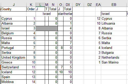
I have tried looking everywhere and cant find anything that works.
Basically this is all of what i need my formula to do:
Example:
-in L3, i want it to check the EB column for the same phrase/value as J3. If it finds it in the EB column, in L3 place the corresponding value of EA column if it finds J3 phrase in EB column
-If EB column doesn't contain J3, rather that return #N/A, I want it to return either nothing or a zero but i still need the same line in the N column to be able to calculate as well as the L column needs to be able to count the total value of all columN L
In the attached image, basically i want the L column to read the following (from L3 down)
-12
-8
-(blank value)
-(blank value)
-7
-5
-(blank value)
-6
-(blank value)
-(blank value)
-(blank value)
-4
-(blank value)
-(blank value)
Hope this makes sense and someone is able to give me some suggestions
- Labels:
-
Excel
-
Formulas and Functions
- Mark as New
- Bookmark
- Subscribe
- Mute
- Subscribe to RSS Feed
- Permalink
- Report Inappropriate Content
May 29 2021 02:45 AM - edited May 29 2021 02:46 AM
In L3:
=IFERROR(INDEX($EA$3:$EA$12, MATCH(L3, $EB$3:$EB$12, 0)), 0)
If you have Microsoft 365, you can also use
=XLOOKUP(L3, $EB$3:$EB$12, $EA$3:$EA$12, 0)
