Simple formula

[jcpolanco]

Hello guys, Please help a brother in need.

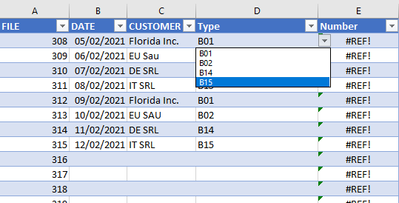
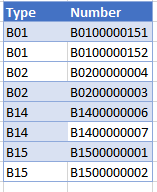
In column D theres a list of 5 items. Whenever i select one of those item it should bring me a number. For instance if i select B01 for row 1 it should bring me the number "B0100000151" and if i select on row 2 B01 again it should brings me the number "B0100000152" which is the next one from B01 type, i would like the same with the other types.

Picture one - Table one

Picture 2 - Table two

Don't hesitate to contact if i need to elaborate

Which formula combination should i use?

[#2]

@jcpolanco Try this:

=[@Type]&TEXT(COUNTIF(Table1[[#Headers],[Type]]:[@Type],[@Type]),"00000000")

[#3]

Thank you so much @Riny_van_Eekelen!

I'm still a bit confused what i should put in the type cells.

=[@Type]&TEXT(COUNTIF(Table1[[#Headers],[Type]]:[@Type],[@Type]),"00000000")

Should it be like this

=[@B01]&TEXT(COUNTIF(table1[[#Headers],[B02]]:[@B14],[@B15]), "number column in table

Maybe better screeshots could help

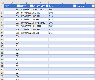
Table one

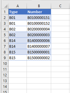
Table two

[#4]

@jcpolanco I have attached the file I worked on. See if you can use it your own file.

[#5]

@Riny_van_Eekelen Thank you Riny so much!! Good input.

The thing is that the table two is static data i just want that whenever i select in column "D" a type for example "B01" i would like that it bring me the number on table two, more specific (column B ;row 2 "B010000151") and then one the second row if i select "B01" again i want it to bring me from table two "B010000152" 

I think it could be done with a VLOOKUP but i don't seem to find the best combination. Also i'm trying to attach the file but doesnt let me.

Am i a bit more clear?

[#6 · Accepted solution]

@jcpolanco I was afraid of that, but you didn't mention it needed to be static so I created a dynamic formula, suspecting that your table would have the all transactions from the beginning for each type (so all start at 1). What you want is not possible with regular formulae, at least I can't think of any. You'd need VBA to lookup the highest number used for a type, increase it by one and dump it in the active cell. VBA is not my thing. Sorry!

[#7]

@jcpolanco

Hi,

I have added formula in Table1. From Column G to Column L I have listed the steps from which it is made. I hope this satisfies your query.