Sequential Conditional Formatting

[mpilon14]

Hello, I am looking to add conditional formatting to my spreadsheet used for inventory tracking. I would like the cell to be highlighted when the amount falls below the specified threshold. I can do this simply for one item and reference the threshold number next to it, but I would like to know how to extend the formula to each item individually, without needing to create a new rule for each item. Right now it seems that when I try to apply the formatting to my other rows, it goes back to reference only the first threshold number (correlating to the first product).

[#2]

@mpilon14 

Please show us what the data look like and what the conditional formatting rule looks like, preferably by attaching a sample workbook.

[#3]

@Hans Vogelaar 

Hello, here is a sample workbook of what I am trying to do. I have a few hundred items I would like to reference their individual re-order threshold and change color when it falls below that number; however, copying the conditional formatting only references the re-order threshold for the first item. In the example, you can see that item C is in red, even though it has not yet reached it's threshold. Is there any way to adjust the formula in the formatting, or do I need to individually add conditional formatting for each item?

[#4]

@mpilon14 

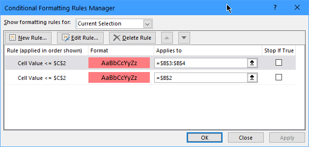
Thank you. The current rule specifies that the cell should be highlighted if the cell value is less than or equal to =$C$2.

$C$2 is an absolute cell reference because of the $ signs. It will not change when you copy the formatting.

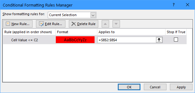
Select B2:B4

Delete the existing rules from the range.

With the range still selected, create a new rule. This time, use relative cell referencing: =C2