Select data within Multiple Rows within date ranges

[markplumridge]

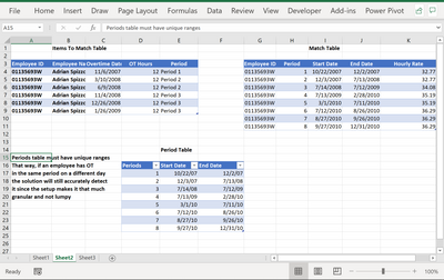
I need to find an hourly rate for an employee the range falls within the date that the overtime was worked.

Here is a sample of the data set

Can somebody help me with a formulae to lookup with both criteria?

[#2]

@markplumridge 

Both criteria? The only criterion that I see described is the date. So let me suggest:

1. that you post not an image but the actual excel file from which the image was taken, so that we (I or somebody else) don't have to go to the trouble of re-creating what already exists. Just make sure there are no real names of real people in the file.
2. that you be a little more specific on what the selection criteria are.

[#3]

@mathetes  Thank you. File is now attached.

[#4]

@markplumridge 

Thank you for posting the spreadsheet. But at first it was more confusing than your original post. The workbook has a front sheet (Sheet1) that contains a few formulas (VLOOKUP and INDEX/MATCH) but they don't refer to the Sheet2, which is where the data you originally posted in image form. Nor is it readily apparent what criteria are being used.

So could you please spell out more clearly what it is you want done with the data on Sheet2 (or Sheet1).

That said, since you specified two criteria at the start, may I point you in the direction of a possible solution. If you have the newest version of Excel, there are some new "Dynamic Array functions," FILTER and UNIQUE among them, that might be the solution you're looking for. Here's a YouTube video that explains them....from the formulas you've written, it would appear that you do have a good grasp of some of the basics of data retrieval from an Excel database.....these new functions take that to a whole new level. https://www.youtube.com/watch?v=9I9DtFOVPIg

But you will need the newest version of Excel for these Dynamic Array functions to work

[#5]

@markplumridge 

I am removing my suggested solution because the suggested solution was only for the presented dataset and not for the 4000 lines of variant [Start Date] and [End Date] for 130 other employees. to get an accurate solution, the [Start Date] column and the [End Date] column must be in a separate table with unique start and end date ranges and must include all date ranges to compare against the 4000 OT dates.  Maybe try @Sergei Baklan solution.

As a variant, here is a sample file for what is being described above.

Where Periods table must have unique ranges

That way, if an employee has OT in the same period on a different day
or a different employee has OT on the same day as 129 other employees the comparison is not looking at multiple instances of the same period range that will skew the result the solution will still accurately detect it since the setup makes it that much granular and not lumpy

See attached

[#6]

Thanks Yea_So
I cant follow your suggestion. I am trying to lookup the hourly rate that the Overtime date falls between so I can use this to calculate a cost using the OT hrs.
Also my actual spreadsheet has over 4000 rows for approx. 130 employees with different range of salary dates so I am unsure how to use your method with this volume of dates.
Hope your can still help!

[#7]

Thanks mathetes. I will take a look and try but it might be beyond my skill set.

[#8]

I'm willing to help more, but you need to give some clarification on exactly what it is you're trying to do,

[#9 · Accepted solution]

@markplumridge 

Based on initial screenshot that could be like

=LOOKUP(2, 1/ ( $G2:$G9 = A2 )/ (C2>=$H$2:$H$9)/ (C2<=$I$2:$I$9), $J$2:$J$9)

For entire range, using dynamic one

=LOOKUP(2, 1/
 ( $G$2:INDEX($G:$G, COUNTA($G:$G)) = $A2 ) /
 ( $C2 >= $H$2:INDEX($H:$H, COUNTA($H:$H)) )/
 ( $C2 <= $I$2:INDEX($I:$I, COUNTA($I:$I)) ),
 $J$2:INDEX($J:$J, COUNTA($J:$J)))

[#10]

Thanks Sergei. That worked.

[#11]

@markplumridge , you are welcome