Second to last value from table with condition

[matt0020190]

Hi experts

Can you help me with the below?

I have a list of cash values in a table, example as follows by a rotating week number (1-4).

A ------------ B

1 ----------- 40

2------------- 30

3------------ 22

4 -----------56

1 -----------33

2 -----------15

3 -----------9

4------------40

1------------18

2------------79

3------------45

4------------61

What I want to do is have a formula to always pick out the second to last value corresponding to the week number. For example if I wanted the second to last value of week 4....

The formula would spit out = 40

If I wanted the second to last value of week 2....

The formula would spit out = 15

I have a formula to get the last value for each week... but second to last I am struggling with. I also need to mention the formula must ignore blank values!!!

Any help appreciated

Matt

[#2]

@matt0020190 

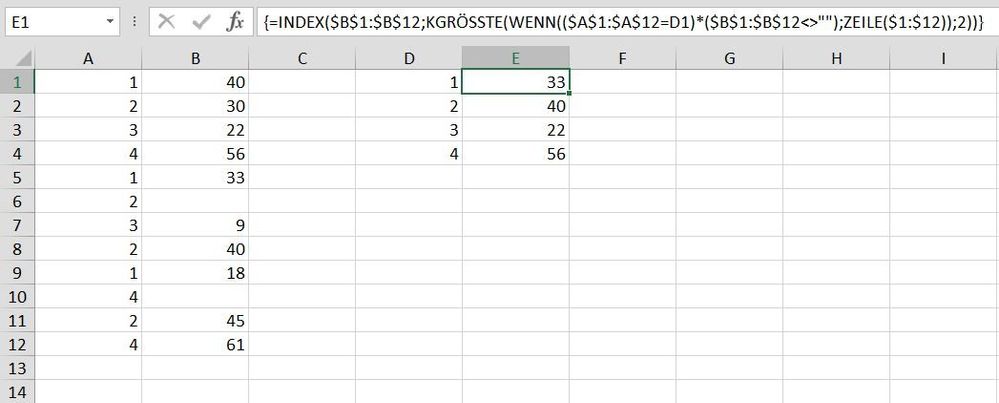
=INDEX($B$1:$B$12,LARGE(IF(($A$1:$A$12=$D$1)*($B$1:$B$12<>""),ROW($1:$12)),2))

Is this what you are looking for? If you don't work with Office365 or 2021 you have to enter formula as arrayformula with ctrl+shift+enter.

[#3]

@OliverScheurich 

Thanks so much for your reply. Sadly haven't got it to work like in your example.

I have knocked up an example spreadsheet. Hopefully this makes sense on how I am trying to use a formula for the second to last value in list?

I also have a formula for last value, this works fine as you will see.

Can you take a look and see what I mean from the cells highlighted in yellow?

Thank you again

[#4]

@matt0020190 

Use

=INDEX($C$6:$C$58,LARGE(IF(($A$6:$A$58=F5)*($C$6:$C$58<>"")*($B$6:$B$58=G5),ROW($C6:$C58)-ROW($C$6)+1),2))

or

=INDEX($C$6:$C$58,LARGE(($A$6:$A$58=F5)*($B$6:$B$58=G5)*($C$6:$C$58<>"")*(ROW($C$6:$C$58)-ROW($C$6)+1),2))

If you don't have Office 2021 or Microsoft 365, confirm with Ctrl+Shift+Enter.

[#5]

Thanks for these.... tried in the example spreadsheet and worked from copy & paste

Then added your formula to my actual spreadsheet by only adjusting the rows/columns to match and now get the #NUM! error

Is this potentially a formatting issue?

[#6]

@matt0020190 

You'll have to adjust the formula for the actual range of course.

If that doesn't work for you, please attach a workbook that better represents your real setup.

[#7]

@matt0020190 

Just in case, this one doesn't require CSE if you are not on Excel 365/2021

=INDEX( $C$6:$C$58, AGGREGATE(14, 6, 1/($A$6:$A$58=$F$5) / ($C$6:$C$58 <> "") *(ROW($A$6:$A$58) - ROW($A$5) ), $G$5 ) )

It's always better to mention Excel version.

[#8]

I am getting #REF! error please help resolve @OliverScheurich 

[#9]

@SatyaGupta_In 

=INDEX($B$1:$B$12,LARGE(IF(($A$1:$A$12=D1)*($B$1:$B$12<>""),ROW($1:$12)),2))

Does this work in your sheet? Enter the formula as an arrayformula with ctrl+shift+enter if you don't work with Office 365 or Excel 2021.

[#10]

how about this？

http://e.anyoupin.cn/bsbm/pdo/eh2/a2502/mybookmark/sql/sql/display_table_t.php?find=+create+temp+tab...

[#11]

downloaded your file, looking good but I am still getting #REF! error, could not attach my Excel file to this reply, please guide @OliverScheurich 

[#12]

@matt0020190 

You need to specify the Excel version.  Otherwise you might get solutions like

= MAP({1;2;3;4},
    LAMBDA(w,
      LET(
        criterion, (week=w)*(amount>0),
        matches,   FILTER(amount, criterion),
        CHOOSEROWS(matches,-2)
      )
    )
  )

A solution written for Excel 365 may have very little in common with earlier generations of spreadsheet.

[#13]

@SatyaGupta_In 

In the screenshot below i've highlighted where you can attach either a file or a screenshot.

[#14]

@matt0020190 

You can use the following formula to get the second to last value for a specific week number:

=INDEX(B:B,MAX(IF(A:A=week_number,ROW(B:B)-ROW(B1)+1)))

Replace week_number with the week number you're interested in.

This is an array formula that uses the INDEX and MAX functions. Here's how it works:

1. IF(A:A=week_number,ROW(B:B)-ROW(B1)+1) creates an array of row numbers where the week number matches week_number. The ROW(B:B)-ROW(B1)+1 part is used to adjust the row numbers to start at 1, since the formula will return an array starting from the first row.
2. MAX(IF(A:A=week_number,ROW(B:B)-ROW(B1)+1)) finds the maximum row number in the array, which will be the row number of the last non-blank cell in the specified week.
3. INDEX(B:B,MAX(IF(A:A=week_number,ROW(B:B)-ROW(B1)+1))) returns the value in column B at the row number found in step 2.

Make sure to enter this formula as an array formula by pressing Ctrl+Shift+Enter instead of just Enter. This will add curly braces around the formula in the formula bar to indicate that it's an array formula.

[#15]

attaching screenshot will not help resolve the issue, please can I not attach the excel file to understand. However, I am attaching link to the file which is residing on my OneDrive.
https://1drv.ms/x/s!Avclfms7aCtXjF0EPX0f_ZClrECh?e=6UTmT3

[#16]

@SatyaGupta_In 

=INDEX(Z1412:Z1761,LARGE(IF((D1412:D1761=M1769)*(Z1412:Z1761<>""),ROW(1412:1761)-1411),2))

Does this return the expected result?

 

[#17]

Thank you very much it is working fine. Can you please suggest a formula for last value based on criteria with if condition based on another column, which works on google sheet as you may know Google Sheet does not accept formula with Filter & Aggregate commands

[#18]

@SatyaGupta_In 

=INDEX(Z1412:Z1761,LARGE(IF((D1412:D1761=M1769)*(Z1412:Z1761<>""),ROW(1412:1761)-1411),1))

Does this return the expected result? I only work with Excel and therefore can only suggest solutions for Excel.

 

[#19]

Thank you sir, it is working but I need formula with if condition based on another column

[#20]

@SatyaGupta_In 

Maybe i can help you with this. Which additional condition do you want and on which column should it be based?