- Home
- Microsoft 365
- Excel
- Re: Rules and conditions specific on each line
Rules and conditions specific on each line
- Subscribe to RSS Feed
- Mark Discussion as New
- Mark Discussion as Read
- Pin this Discussion for Current User
- Bookmark
- Subscribe
- Printer Friendly Page
- Mark as New
- Bookmark
- Subscribe
- Mute
- Subscribe to RSS Feed
- Permalink
- Report Inappropriate Content
Nov 14 2022 04:38 PM - edited Nov 14 2022 07:24 PM
Hello,
I'm having issues with some conditions. I have employees that are younger than others in the company and I need to check when I have to control their work (juniors needing to be tested more often than seniors).
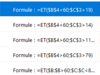
Therefore I have 3 rules for Jr and 3 rules for Sr as shown on the screen shot : screenshot
In the E column I have the date when I checked their work. If it's more than 20 days for jr, their names and forenames goes red. If more than 15 days, it goes orange (as a reminder).
It's the same for Sr but every 111 days (red) and 80 days (orange).
I have their first day in the company in the B column and the number of days since (to determine if he/she has been in the company for more or less than 60 days) to know which 3 rules to apply.
According to their arrival date, a different rule will apply.
So far, my rules have been working for the first employee in every possible combinaison, but here is my issue:
I would like to have these 6 rules applied for every employee automatically on each line, accordingly to their own dates (since they all came in the company on a different day and their last check-up isn't on the same day neither), without having to re-enter each rule manually. If a new employee comes in my sheet, I'd like the rules to apply directly.
When I set the rule range (all the cells the rule must apply) to all the A column, it bases the rules only on the dates and conditions from the first employee, which is wrong since every employee has a different date for their last check-up and their arrival into the company.
Does anyone know how I can deal with this, to apply the rules accrodingly to the line it's on with specific dates without having to set all the rules manually ?
Thank you so much for your help!
- Labels:
-
Excel
-
Formulas and Functions
- Mark as New
- Bookmark
- Subscribe
- Mute
- Subscribe to RSS Feed
- Permalink
- Report Inappropriate Content
Nov 14 2022 06:34 PM
Solution
In the screen shot you have absolute references; they need to be relative, in order for the conditional formatting in the lower rows to be using data from that respective row. So change $B$4 to B4 (or at least $B4); Similarly the reference to $C$3, although it's not clear to me why that refers to a different row. Of course, I don't know how you've arrayed the data for each employee.
- Mark as New
- Bookmark
- Subscribe
- Mute
- Subscribe to RSS Feed
- Permalink
- Report Inappropriate Content
Nov 14 2022 07:23 PM
- Mark as New
- Bookmark
- Subscribe
- Mute
- Subscribe to RSS Feed
- Permalink
- Report Inappropriate Content
Nov 15 2022 08:01 AM
I don't know why excel decided to put the cell I was clicking on in absolute...
Yes. That's the default way it works. I've been caught in that trap myself, which is why I knew to look there first.
Accepted Solutions
- Mark as New
- Bookmark
- Subscribe
- Mute
- Subscribe to RSS Feed
- Permalink
- Report Inappropriate Content
Nov 14 2022 06:34 PM
Solution
In the screen shot you have absolute references; they need to be relative, in order for the conditional formatting in the lower rows to be using data from that respective row. So change $B$4 to B4 (or at least $B4); Similarly the reference to $C$3, although it's not clear to me why that refers to a different row. Of course, I don't know how you've arrayed the data for each employee.
