Return the column next to the top 3 values

[LucyK]

Hi!

I would like to return the name of a column, if it is in the top three. So for example:

Best Dept	10
Good Dept	8
OK Dept	8
Meh Dept	7
Bad Dept	6
Awful Dept	5

I want the names of the top 3 departments (so in this case, best, good, and OK) against the metric. 

I can see how to use LARGE to identify what the top 3 numbers are, but I can't work out how to take that reference, and move one column to the left, to give the name. 

Using MATCH or VLOOKUP doesn't work, because the metric isn't always unique - in this case good & OK both have a score of 8, so if I use MATCH I only get Good listed. 

I've tried using CELL and OFFSET but both give me errors, and I can't seem to fix them. 

Any help is appreciated!

[#2 · Accepted solution]

@LucyK 

If you have Microsoft 365 or Office 2021, enter the following formula in a cell. It will spill to three cells automatically.

=FILTER(A2:A7, B2:B7>=LARGE(B2:B7, 3))

The following will work in any version. Enter the following formula in F2 and confirm with Ctrl+Shift+Enter, then fill down to F4.

=INDEX($A$2:$A$7,MATCH(1,($B$2:$B$7=LARGE($B$2:$B$7,ROW()-1))*(COUNTIF($F$1:$F1,$A$2:$A$7)= 0),0))

See the attached sample workbook.

[#3]

@LucyK 

The new FILTER function will work for this (it does require the newest version of Excel, however).

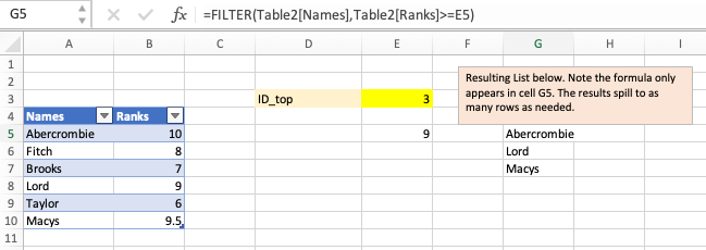
I've created an example for you in the attached. You pick the number in the yellow cell (i.e., the top 1, 2, 3, etc), LARGE will identify the metric associated, and FILTER will pick all of the departments that meet or exceed that metric.

Just to make it fully dynamic, I created a Table ("Table2" in the formulas) with "Names" and "Ranks" as the headers for the two columns (you'll see those referred to in the formulas below). Creating this as a table allows you to add rows indefinitely and still enable the formulas to work. And I named the yellow cell "ID_top", which you'll also see in the formula referring to it.

=LARGE(Table2[Ranks],ID_top)    

=FILTER(Table2[Names],Table2[Ranks]>=E5)   E5 is the cell where the boundary rank is displayed

I hope you notice, too, that the scores do not need to be sorted in order.

[#4]

Thank you!