- Home
- Microsoft 365
- Excel
- Re: Retrieving Full Rows For Any Cells Matching Search Query
Retrieving Full Rows For Any Cells Matching Search Query
- Subscribe to RSS Feed
- Mark Discussion as New
- Mark Discussion as Read
- Pin this Discussion for Current User
- Bookmark
- Subscribe
- Printer Friendly Page
- Mark as New
- Bookmark
- Subscribe
- Mute
- Subscribe to RSS Feed
- Permalink
- Report Inappropriate Content
Dec 30 2021 01:04 PM
Hi! I use Spreadsheets for pretty basic stuff but have been trying to get into more complex uses for my new job. Something I'm setting up is a database for customer calls we receive, cataloguing their names, numbers, emails, complaints, etc., and I'd like to implement a search function where information entered into a specified cell will pull full rows that contain the query in any of its cells.
I formulated the following into a test document after doing some reading online (note I haven't applied ISERROR yet because I'm taking this formula step by step in order to understand it as fully as possible.):
=INDEX($A$2:$D$10,SMALL(IF($A$2:$D$10=$B$12,ROW($A$2:$A$10)),ROW(1:1))-1,0)
The thing is, for various reasons I've been using open source programs such as LibreOffice at home and am re-orienting toward Excel since my job uses it extensively. When plugged into LibreOffice (I selected cells A15:D15, applied formula with Ctrl-Shift-Enter, Ctrl-dragged down), the above formula gave me exactly what I want: a query in cell B12 brings up the full rows of information for any cells containing the query.
When I brought this over to Excel, the same formula only pulls the first column of data and repeats it across the row.
Is there a way to modify this formula to mirror the results I got in LibreOffice, or is there another method I must implement to get the same results?
Excel version:
Microsoft® Excel® for Microsoft 365 MSO (Version 2111 Build 16.0.14701.20240) 32-bit
PC:
Windows 10 Pro
I would attach the test file as suggested but I can't find an explanation of how to do that on this site.
Much appreciated!
- Labels:
-
Excel
-
Formulas and Functions
-
Office 365
- Mark as New
- Bookmark
- Subscribe
- Mute
- Subscribe to RSS Feed
- Permalink
- Report Inappropriate Content
Dec 30 2021 01:58 PM
=INDEX(A$2:A$10,SMALL(IF($C$2:$C$10=$B$12,ROW($A$2:$A$10)),ROW(1:1))-1)
Is this what you want to do? As you work with Office365 you can as well use FILTER formula.
- Mark as New
- Bookmark
- Subscribe
- Mute
- Subscribe to RSS Feed
- Permalink
- Report Inappropriate Content
Dec 30 2021 04:02 PM
- Mark as New
- Bookmark
- Subscribe
- Mute
- Subscribe to RSS Feed
- Permalink
- Report Inappropriate Content
Dec 31 2021 07:52 AM
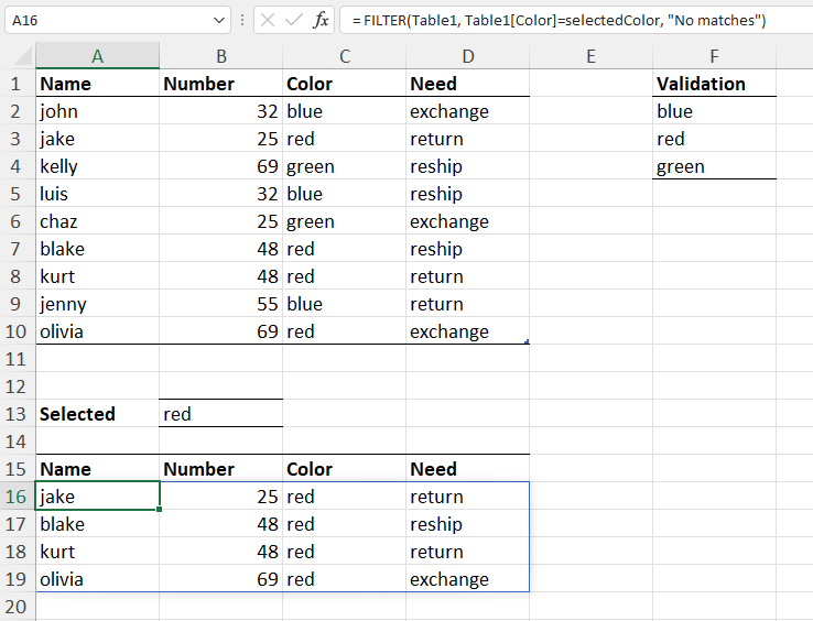
If without sorting I'd filter with headers
=FILTER(
     Table1[#All],
    ( Table1[[#All],[Color]] = selectedColor ) +
    ( Table1[[#All],[Color]] = Table1[[#Headers],[Color]] ) )
Still works if sort by Numbers.
- Mark as New
- Bookmark
- Subscribe
- Mute
- Subscribe to RSS Feed
- Permalink
- Report Inappropriate Content
Dec 31 2021 11:36 AM
@OliverScheurich @Peter Bartholomew @Sergei Baklan Thanks for the replies! It looks like FILTER mixed with smart use of Tables is going to be the way to go, and I've been learning a lot through the examples shown here & messing around in a more complex test document to make sure the function works for as many use cases as possible.
I'm still having issues attaching files on this site, will try to figure it out to provide the document I'm messing with because I think it will make it very clear what my aim is, but I wanted to give an update on the formula I have been working with and describing how it's working for anyone who might stumble upon this discussion.
The first thing I did was create a table out of a larger set of data that my first example, designating columns for date, first name, last name, email, phone number, product purchased, and call details which contain duplicate entries in every column.
I then used FILTER to reference each column of the table individually against a single cell (in my document it's cell E3), like such:
=FILTER(Table,
(Table[Column1]=E3)+
(Table[Column2]=E3)+
(Table[Column3]=E3),"")
This accomplishes most of what I'm looking for! I am still learning the Excel syntax and operators, the plus sign (+) designates "OR" so Excel is looking at my query and thinking "does it match Column 1 or Column 2 or Column 3 or etc?" which is the kind of designation I was looking for, since a lot of functions seem to only work with single rows or columns. With this, rows will be pulled if any cell in any column is an exact match.
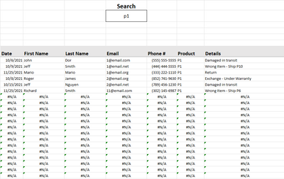
Product Search:
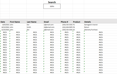
First Name Search:
Date Search:
With this setup, the only roadblocks I am encountering are that I can't get partial matches to work (tried ISNUMBER and SEARCH but kept getting popup errors), I can't the list of #N/As that you can see above to remain blank (IFERROR, IFNA, ISERROR, etc don't get rid of them/give me popup errors), and queries with a single result will repeat down the list:
Some of these might just be the limitations of this kind of software/logic, in which case this is still functional for my needs and I can either adjust what I'm trying to do to accommodate or just live with it haha. I got further than I expected with the great help here! When I get home I will try to upload the file again, might be an issue with the network at work or I might be missing something but I can't find another way to attach a file aside from drag & drop which isn't working on this machine.
Thanks again!
- Mark as New
- Bookmark
- Subscribe
- Mute
- Subscribe to RSS Feed
- Permalink
- Report Inappropriate Content
Dec 31 2021 02:20 PM
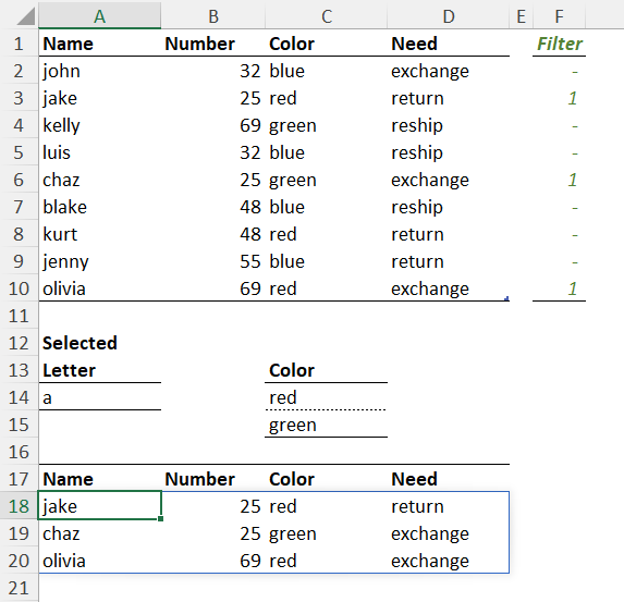
As you suggest, more complex criteria may be implemented using "+" for OR and "*" for AND. For example, the formula
= FILTER(
     Table1,
     ISNUMBER( SEARCH(selectedLetter, Table1[Name]) )
        * ((Table1[Color]=selectedColor1)+(Table1[Color]=selectedColor2)),
     "No matches"
  )
returns any record with a name containing an "a" and colors red or green.
- Mark as New
- Bookmark
- Subscribe
- Mute
- Subscribe to RSS Feed
- Permalink
- Report Inappropriate Content
Jan 01 2022 02:51 AM
Another pattern is to use COUNTIF()
= FILTER(
      Table1,
         ISNUMBER( SEARCH(selectedLetter, Table1[Name]) ) *
         COUNTIF(selectedColors, Table1[Color]),
       "No matches")


