Replace #N/A with prior available values on a 2D running array with ONE "spill" formula

[leolapa]

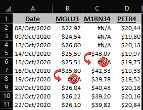
Below is a small sample from close market prices for 3 stock tickers using the STOCKHISTORY function:

I realized that when no data is available for a particular stock, it then returns the #N/A error.

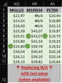
The problem for me is that it screws up my day-to-day % variance calculation, among other things, so I want to replace those #N/A's with the last available trading day's price, like the screenshot below:

But here's the catch: only a single-cell "spill" formula will work for me. On the above screenshot, it needs to be a formula on cell "AQ2" that "spills" the values down and across, the same way the STOCKHISTORY function works.

Since I don't know a way to make the STOCKHISTORY function do that #N/A replacement job in and of itself, albeit it would be GREAT if it could, I had to find a workaround to make that happen for me.

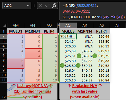
So I did a couple of calculation steps in order to get the row numbers array that would serve as input to the final INDEX function, and managed to get to a 1D "spill" solution for each of the 3 individual tickers columns on that example, as shown below (I just don't know how to trick those 3 yellow-shaded validation arrays into one consolidated formula without returning error):

The couple areas highlighted in red indicate the rectified row numbers that will serve as replacements for the #N/A's that have prior values to be used on their places.

However the formula

=LET(Acumul_Range;$F$2#;Rows_Range_Seq;SEQUENCE(ROWS(Acumul_Range));Cols_Range;COLUMNS(Acumul_Range);--MID(BYCOL(1;LAMBDA(Agreg_Range;CONCAT(TEXT(MOD(SMALL((Rows_Range_Seq*100000)+(SEQUENCE(;Cols_Range)*(Acumul_Range=Agreg_Range));Rows_Range_Seq*Cols_Range);100000);"0000"))));(Rows_Range_Seq*4)-3;4))

only treats each column individually, and that's the piece that I'm missing to get to my final goal...

... which is the formula

=INDEX($B$2:$D$11;$AM$2:$AO$11;SEQUENCE(;COLUMNS($B$1:$D$1)))

 that produces the final array previously shown:

If I can get that row number formula to work down and across a 2D range, then I would be able to replace that "$AM$2:$AO$11" piece of the INDEX function with the hash reference "$AM$2#" and therefore get this baby kicking and screaming across the finish line.

Any ideas/suggestions on how to finesse that intermediate formula?

Thanks in advance...

[#2]

@leolapa 

Consider using IFERROR formula

=IFERROR(YourFormula,PreviousCellValue)

=IFERROR(INDEX($B$2:$D$11;$AM$2:$AO$11;SEQUENCE(;COLUMNS($B$1:$D$1)));C2)

=IFERROR(YourFormula,C2)

[#3]

@leolapaGive the below a try, leverages MAKEARRAY as in previous solution.

=LET(
    rng,B2:D11,
    MAKEARRAY(
        ROWS(rng),
        COLUMNS(rng),
        LAMBDA(i,j,
            IF(
                i=1,INDEX(rng,i,j),
                IFERROR(INDEX(rng,i,j),INDEX(rng,i-1,j))
            )
        )
    )
)

[#4]

That solution would indeed work just fine in case it was 100% guaranteed that STOCKHISTORY would return only one consecutive date with #N/A.
However in real world there might be occasions where #N/A may show up in two or more consecutive dates, and in those cases that solution would still return #N/A since it doesn't look up for the valid price from the last available date.

[#5]

I tried to apply that solution just as you did, but the thing is that it only addresses cases with only one instance of #N/A, since it just pulls the value from one row above.
Since there might be instances where STOCKHISTORY will return two or more consecutive dates with #N/A, how can I adapt that solution so it will look for the price from the last available date? A recursive LAMBDA approach? And if so, how to setup the exit path so the formula will return no error? Still wrapping my head around that...

[#6]

Can you try using some sample where it will occur?

[#7 · Accepted solution]

@leolapa  Ahh, sorry, misunderstood. This solution handles that case, however if the very first entry is an error, it will show the errors; only if there is a prior non-error value in the column will it show the value.

=LET(
    rng,$B$2:$D$11,
    rows_,SEQUENCE(ROWS(rng)),
    nonerror_rows,--(NOT(ISERROR(rng)))*rows_,
    working_rows,
        MAKEARRAY(
            ROWS(nonerror_rows),
            COLUMNS(nonerror_rows),
            LAMBDA(i,j,
                MAX(
                    1,
                    IF(
                        i=1,INDEX(nonerror_rows,i,j),
                        MAX(
                            INDEX(nonerror_rows,SEQUENCE(i),j)
                        )
                    )
                )
            )
        ),
    INDEX(rng,working_rows,SEQUENCE(,COLUMNS(rng)))
)

This is very similar to my answer on your prior post for last matching row.

[#8]

Thanks a lot!!!

[#9]

The thing is that your proposed approach contains one "static" cell within it (in that case, C2), so my understanding is that requires it to be dragged along down and across whatever range size I'm dealing with, so since it's not a one-cell "spilled" type solution it won't work for me, as my goal is to provide a solution that will deal with a growing table (both in columns - that is dates, and rows - that is stock tickers).

[#10]

@leolapa 

Just for the interest recursion solution. Not very practical since max about 300 rows spill size.

FillDown = lambda(array, [m],
    LET( n, IF(ISBLANK(m), rows(array), m),
        IF( n = 1, INDEX(array, 1),
            LET( a, FillDown(array, n-1),
                IF( SEQUENCE(n) < n, a,
                    IFNA(INDEX(array, n ), INDEX( a, n-1) )
                )
            )
        )
    )
);

and

=FillDown(STOCKHISTORY($C$1,A2,A2+300,0,0,1))