Regarding the filter by condition option in pivot table in the excel

[BHARGAV_RAM_D_R]

I'm taking Google Data analytics course in the coursera, there they use filter in the pivot table and apply conditions like, less than or greater than, they were using the Google sheets, and I couldn't find that option in the excel, you can select or unselect the value in the filter but there's no option to apply conditions like lesser than or greater than such value. Is there any way you guys know, from which you filter the fields by conditions, please let me know.

[#2]

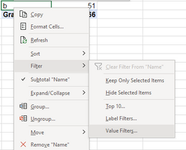
@BHARGAV_RAM_D_R I'm not familiar with Google sheets, but in an Excel pivot table, right-click anywhere on a row label. Choose Filter, Value filters...

No you can select the type of filter as you described in your question.

[#3]

@Riny_van_Eekelen Thank you for this tip! 

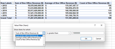
@BHARGAV_RAM_D_R I'm in the same course, and had the same issue. It won't work if you right-click one of the years and then apply the filter as @Riny_van_Eekelen explains. This is because the filter is then applied to the years (summary) values rather than to each individual movie's (non-summary) value. See how the window below is labeled "Value Filter (Years)"?

To fix this, you need to apply the filter to each individual movie (individual rows in the original data).

Making Individual Movie Releases Visible 

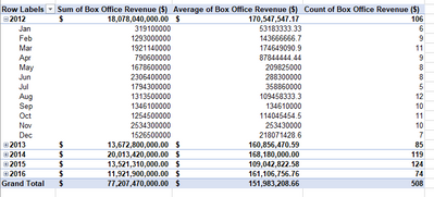
My pivot table wasn't showing individual movies by default -- just summary values for years and months, like this:

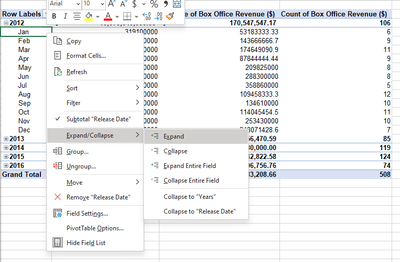
So I had to get it to show more detail. To do this, simply right-click one of the months > Expand/Collapse > Expand > choose a field.  

I didn't really think it mattered which field I chose, and showing the movie title seemed like a more realistic way to look at data in real life so I chose that. Then my table looked like this:

Add Value Filter to Only Show Individual Releases <$10M 

At this point, I was ready to filter by individual movie releases (individual rows in the original table). So I right-clicked one of the movie titles > Filter > Value Filters. Now, you'll see that the title of the pop-up window is "Value Filter (Movie Title)." Here, I chose Sum of Box Office Revenue ($) (you'll need to choose choose SUM <$10M if you've already renamed your fields) | is less than | 10,000,000 (commas optional). Like this:

(Note: If you right-click a year or month, it will filter at that level. This would be useful if you wanted to only see data for years/months where you made less than $X, but it's not what we're looking at in this exercise.)

Now, the pivot table is updated. The updates hold even if you collapse your view to only show the summary data by year. This is because you have filtered by the individual movie rather than the entire year. 

Now, you'll see a down-arrow on the row label title (A3 for me). To remove the filter, you'll need to again click on the correct level (any movie title for this example), then click the filter icon (down-arrow) and then click Clear Label from 'Movie Title'. Updating works similarly.

You could even add a filter at the month or year level (e.g., only show movies where the total annual revenue was <$X). Or combine a year filter with the existing movie title filter you just created (e.g., only show movies with revenue <$10m in years where the total annual revenue was <$X).

It's definitely less intuitive than the Sheets filtering options, but it's pretty easy to work out once you get a sense of how it's all set up.  I hope this helps someone else!