- Subscribe to RSS Feed
- Mark Discussion as New
- Mark Discussion as Read
- Pin this Discussion for Current User
- Bookmark
- Subscribe
- Printer Friendly Page
- Mark as New
- Bookmark
- Subscribe
- Mute
- Subscribe to RSS Feed
- Permalink
- Report Inappropriate Content
Jul 07 2021 12:08 PM
I would like to have Column P rank the players relative to their position. To clarify, Devante Adams in A7 has an Average Rank of 6 (found in O7), yet is the #1 WR (position shown in Column B). So, the value in P7 should be 1. Then, if Stephon Diggs in A9 has an average rank of 8 (found in O9), the value in P9 should be 2. This is because he has the second highest average rank of all players with "WR" in Column B. How can I do this?
- Labels:
-
Excel
- Mark as New
- Bookmark
- Subscribe
- Mute
- Subscribe to RSS Feed
- Permalink
- Report Inappropriate Content
Jul 07 2021 02:12 PM
Solution
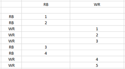
This is a little tricky. I would add some helper columns for each position to help track. You'll have to change the columns around but something like this should work.
In the helper columns:
=IF($O195=P$193,1+COUNT(P$194:P194),"")
It'll count each occurrence and rank them in order. From there, you'll need to do another xlookup for each player like in your previous question.
Let me know if you can work this to fit your workbook or if you need more explanation!
Accepted Solutions
- Mark as New
- Bookmark
- Subscribe
- Mute
- Subscribe to RSS Feed
- Permalink
- Report Inappropriate Content
Jul 07 2021 02:12 PM
Solution
This is a little tricky. I would add some helper columns for each position to help track. You'll have to change the columns around but something like this should work.
In the helper columns:
=IF($O195=P$193,1+COUNT(P$194:P194),"")
It'll count each occurrence and rank them in order. From there, you'll need to do another xlookup for each player like in your previous question.
Let me know if you can work this to fit your workbook or if you need more explanation!


