- Subscribe to RSS Feed
- Mark Discussion as New
- Mark Discussion as Read
- Pin this Discussion for Current User
- Bookmark
- Subscribe
- Printer Friendly Page
- Mark as New
- Bookmark
- Subscribe
- Mute
- Subscribe to RSS Feed
- Permalink
- Report Inappropriate Content
Apr 23 2019 04:09 AM
Hello,
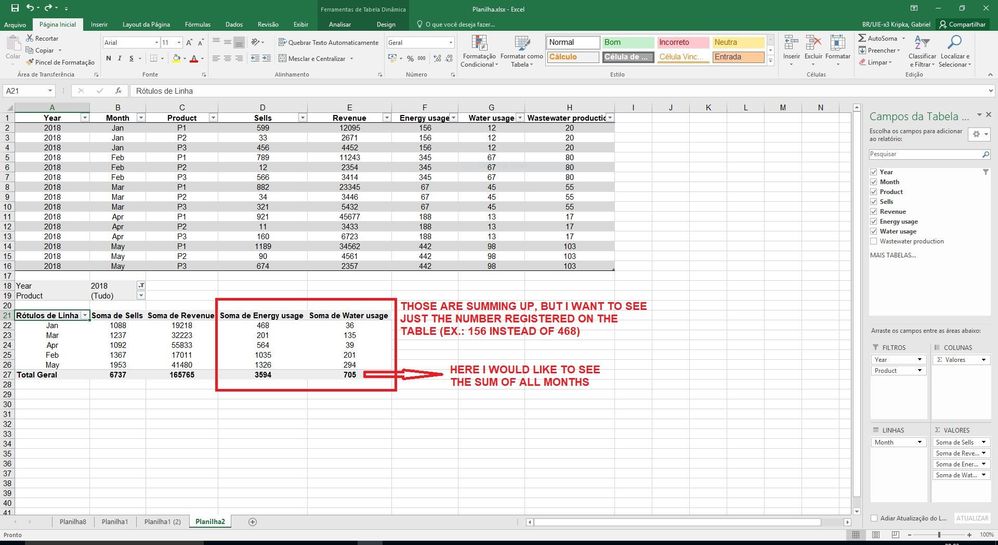
I am facing a problem with data arrangement in a pivot table. When configuring my data base table, the lines are composed of 3 products, while the columns contain information about number, cost etc. One column contains the month, and I have to repeat each month 3 times down to include the 3 products each month. Some other columns involve numbers that are not related to a specific product and therefore I just equally repeat the number 3 times.
In the pivot table (which is set to present the months as lines), the sum of this repetition gives me the obvious result of a x3 multiplication, however I would like to receive only the number itself, but without setting the results to “count”, “maximum” or “minimum”, because I want the final line in the pivot table to give me the sum for all months.
Prints are attached to this description.
Thank you so much
Gabriel
- Labels:
-
Pivot tables
-
Tables
- Mark as New
- Bookmark
- Subscribe
- Mute
- Subscribe to RSS Feed
- Permalink
- Report Inappropriate Content
Apr 23 2019 07:54 AM
@GbiKripka28
Olá Gabriel!
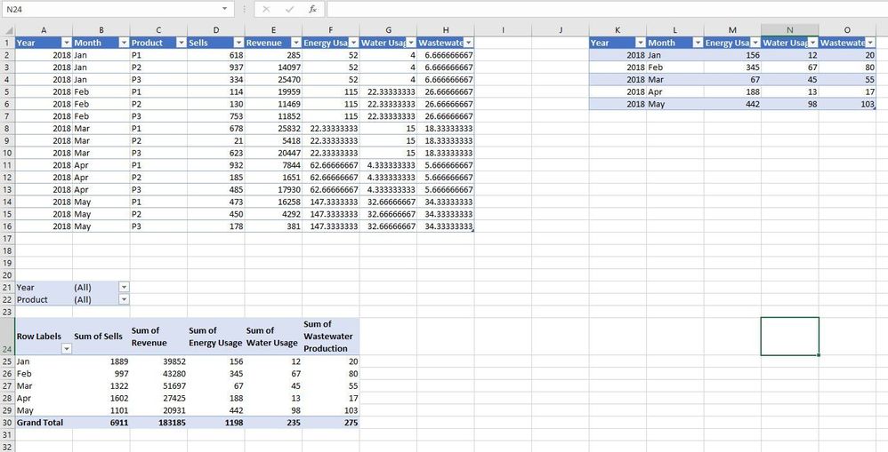
One good solution would be to have a separate table with the energy and water consumptions per month (one row per month.) Then we would use Power Pivot to connect those two tables and that would allow us to create on pivot table grabbing information from those two data tables. I am leaving this tip here in case you want to explore the idea of learning Power Pivot.
Without that option, you could still set the water and energy costs on a separate table and then bring those values to your main table, divided by the number of products you have each month.
For example, for the energy usage, th formula would be:
=SUMIFS(Table2[Energy Usage],Table2[Year],[@Year],Table2[Month],[@Month])/COUNTIFS([Year],[@Year],[Month],[@Month])
where table 1 is your main table and table 2 is the table with the water and energy costs.
Please also see file attached.
I hope this helps.
Votos de um dia feliz! :)
- Mark as New
- Bookmark
- Subscribe
- Mute
- Subscribe to RSS Feed
- Permalink
- Report Inappropriate Content
Apr 23 2019 07:54 AM
Hi Gabriel,
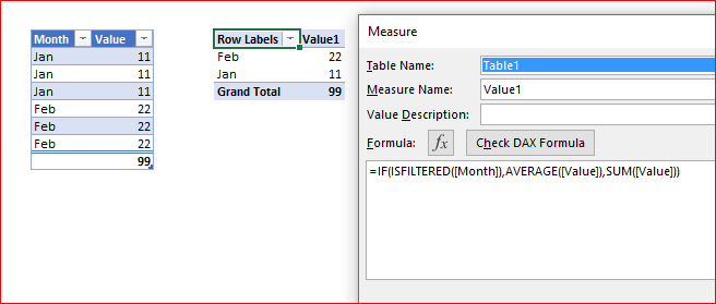
If you added data to data model creating the PivotTable, you may add measure like this
and use it instead of the column pivoting the table
- Mark as New
- Bookmark
- Subscribe
- Mute
- Subscribe to RSS Feed
- Permalink
- Report Inappropriate Content
Apr 23 2019 09:12 AM
Thank you for your assistance. How can I "add data to data model" when creating the pivot table? I do not understand a lot from pivot tables. The worksheet you sent is exactly what I was looking for, but how may I reproduce it in my sheets?
Thank you so much
Gabriel
- Mark as New
- Bookmark
- Subscribe
- Mute
- Subscribe to RSS Feed
- Permalink
- Report Inappropriate Content
Apr 23 2019 09:32 AM
Gabriel,
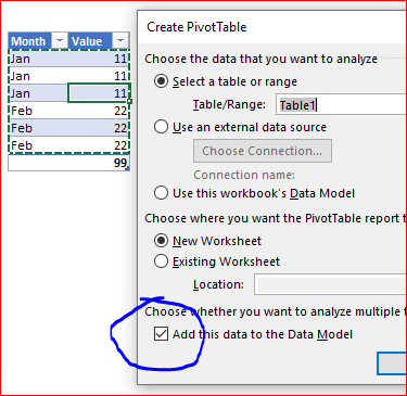
Perhaps you already here, that's default option in recent versions of Excel. However, creating new PivotTable be sure what setting is checked
For the existing PivotTable simplest way to check is right click on the table here
If you see Add Measure you work with the data model.
If not, click on More tables and Yes after that to add your existing data to data model.
New PivotTable will be created using the same layout as existing one, however you may lost all formatting. Remove old one and move new on the desired place.
After that right click on table name, select Add measure and in window as in previous post add DAX formula like
=IF(ISFILTERED([Month]),AVERAGE([Value]),SUM([Value]))
using your actual column names. Aggregate your pivot table using this measure instead of the column.
- Mark as New
- Bookmark
- Subscribe
- Mute
- Subscribe to RSS Feed
- Permalink
- Report Inappropriate Content
Apr 24 2019 06:24 AM - edited Apr 24 2019 06:25 AM
- Mark as New
- Bookmark
- Subscribe
- Mute
- Subscribe to RSS Feed
- Permalink
- Report Inappropriate Content
Apr 24 2019 06:55 AM
Good luck! If you're interested I can recommend some great courses. Let me know if you'd like that.
In the meantime, if you want, you can use the file that I built for you. It solves your problem.


