Predefined Text in Cells

[ituryu]

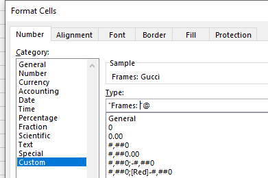
Hi there. Does anyone know if it's possible to have predefined text in cells that only becomes visible after you type in it.

For example I label a column as frame, and in every cell of that column, I could type "GUCCI" but what I want to now appear is FRAME: GUCCI, thus the FRAME: precedes the actual name of a designer frame.

Thus will this be in custom format and how can I go about doing this.

Thanks. 

[#2]

Hi @ituryu

How about this...

[#3]

Hi,@Wyn Hopkins 

I am truly grateful, thanks a gazillion, it worked exactly.

Cheers.

[#4 · Accepted solution]

No worries @ituryu 

Wyn

MVP

Australia UTC+ 8

If this answer was the best response please click the button

I also happily accept likes

[#5]

Hello,@Wyn Hopkins 

Thanks for the great pointer, but I seem to have developed an unexpected change and I'm not too sure what to do to rectify it. After using the custom "FRAME:" @ formatting, my sumifs function to help compute my weekly sales stopped working! I've tried inputting the custom format in the text reference but still not computing. So I'm guessing my syntax in wrong but not sure what next to do.

=SUMIFS($G$4:$G$359,$A$4:$A$359,">="&AE25,$A$4:$A$359,"<="&AF25,$F$4:$F$359,$AJ$23&": *")

Please help!!! That's the formula I used.

Thank you.

[#6]

Hi

I can't really tell from just the formula, but at the end it references ": *" " if that is referring to the FRAME: GUCCI then it won't work since " : " is just part of the formatting not actually part of the result

[#7]

Hi,@Wyn Hopkins 

Please what do you suggest that I do to get this resolved cause I've tried deleting it and also tried replacing as a text, but it isn't calculating!!!

 Any creative ideas from your noble end please?

[#8]

Could you attach a sample / example file and I’ll take a look

[#9]

Hi, 

Yes this is a sample file you can assist with. The weekly sales summary frame section is where lies the problem.

Thanks.

[#10]

@ituryu 

Parallel discussion on exactly the same topic is here https://techcommunity.microsoft.com/t5/excel/weekly-summary-malfunction/m-p/1130195

[#11]

You need to physically type Frames: into your cells for your SUMIFS to work

Personally I'd add separate columns to hold the words you are searching for Lenses and Frames rather than putting the prefix on the description.  Also add data validation  so you don't accidentally spell something wrong and therefore not pick up the correct value

Wyn

[#12]

@Wyn Hopkins 

I like the number formatting.  The text field is one that I have rarely used.  I guess it could get interesting combined with conditional formatting.

As for the OP question

= SUMIFS( FramesCost, Date,">="&WeekStart, Date,"<="&WeekEnd, Frame, "<>")

simply testing for non-blank fields should achieve the objective.

[#13]

Hi,@Peter Bartholomew 

I gave it a trial but ended up with no sum, I had to remove the custom format as I was getting #NAME! error returned!!!

[#14]

@ituryu 

Custom format affects nothing in SUMIFS, you may keep it

[#15]

Hello,@Sergei Baklan 

I have removed it and the formula is now working fine! I truly would loved to keep the custom format on the frame but nothing seems to work except I take out the custom format. Please how do I resolve this and move forward w/ this sheet as I have a deadline.

Thanks and cheers.

[#16]

@ituryu 

Perhaps I misunderstood something. Did you modified SUMIFS? Could you please submit working sample for better understanding.

[#17]

@Sergei Baklan 

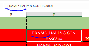
No I did not modify the SUMIFS formula, all I did was remove the custom format from the frame column, i.e, the ("FRAME": @ ) I removed and left that section as general!

Also find attached the working sample you requested for.

Thank you so much for the assistance.

Cheers.

[#18]

@ituryu 

As @Sergei Baklan pointed out, the use of a number format makes no difference to the cell content.

My use of names requires one to define the Names, something that Bill Bricklin (the inventor of the electronic spreadsheet) described as 'tedious'.  Using direct cell referencing, the following works, with or without the custom format:

=SUMIFS($G$4:$G$359,$A$4:$A$359,">="&AE24,$A$4:$A$359,"<="&AF24,$F$4:$F$359,"<>")

[#19]

@ituryu 

I see, you removed it from custom formatting and added FRAME to the cells values

Thank you for updating with this info.