Power Pivot values based on criteria

[ahhk2000]

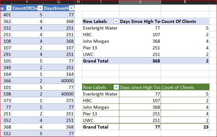
Hi Forum, advice appreciated on this situation based on the attached sheet. I made this sample on a Mac (no Power Pivot in Excel) , the actual situation is at work with a large data model involved. 

Rather than showing the days since last service interaction, I want to show days since last High Touch interaction. Here I can just set a filter, but in the real use case, the pivot table is a dashboard where other values should be based on full data set. 

Rather than counting clients, I want to count only the clients with 2 or more service interactions. 

What would be the sensible approach?

[#2 · Accepted solution]

@ahhk2000 

If without data model you may add two helper columns

as

=COUNTIFS([Company],[@Company])

and

=MIN(TODAY()-MAXIFS([Service Date],[Service Type],"High Touch",[Company],[@Company]),40000)

With that you may add slicers on these fields and move somewhere away, e.g. into separate hided sheet. 

If you shift on Windows or one day Power Pivot appears on Mac, you may add two measures and use them in PivotTable (green one)

Count of Clients:=VAR cnt=COUNTROWS(Table1)
VAR DaysSince=CALCULATE(
       TODAY()-MAX(Table1[Service Date]),
       FILTER(Table1, Table1[Service Type]="High Touch")
)
RETURN
    IF( OR(DaysSince=TODAY(), cnt<2), BLANK(), cnt)

and

Days since High Touch:=VAR cnt=COUNTROWS(Table1)
VAR DaysSince=CALCULATE(
       TODAY()-MAX(Table1[Service Date]),
       FILTER(Table1, Table1[Service Type]="High Touch")
)
RETURN
    IF( OR(DaysSince=TODAY(), cnt<2), BLANK(), DaysSince)

[#3]

Thank you so much for the detailed and informative feedback. Very grateful for your help! @Sergei Baklan 

[#4]

@ahhk2000 , you are welcome, glad to help