Plot isn’t showing up on my chart in excel

[Roger1981]

Hello everyone!

Need your guidance for the below pls.

1. Device and OS Platform: Mac/macOS Big Sur version 11.4

2. Excel product name and version number: Office 365 and 16.50(21061301)

3. Problem encountered:
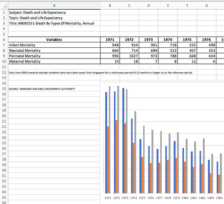
I’m trying to create a simple chart and multi graph using the data from the attachment. Specifically, I’m trying out the data from sheet T3.

I have no problem creating a chart from window OS. I.e., age group (y-axis) against year (x-axis). However, whenever I use Mac OS to create the graph using the same data selection and setting, the chart's plot simply doesn’t show up.

In addition, the “recommended chart” function also doesn’t work.

Please kindly advise.

[#2 · Accepted solution]

@Roger1981 Can't really tell what happened but the numbers in the table weren't recognised as such. They were seen as texts and could thus not be plotted.

Check it in your own file. Type =ISNUMBER(cell) somewhere and points any of the "numbers" in the table. It comes out FALSE, meaning it's not a number.

I entered a formula like =VALUE(B7) in B7 below the graph and copied it four rows down and 49 columns to the right. Then formatted the original data range to "Number" and copied/pasted values from the range with the VALUE formulae on top of the original data range. 

See attached.

[#3]

Thank you.

Indeed, it was the format of the cell causing this issue. It wasn’t number at all.

The problem is solved and I learnt something new.

Thank you so much and appreciate it.