Please Help With this Excel Problem!

[lanem1010]

Hi,

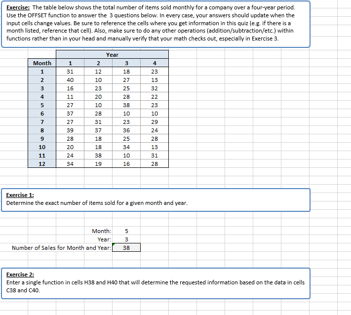
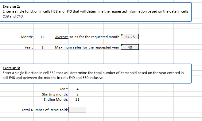
I am trying to solve this last part to the problem and cannot seem to find a correct answer. I have attached both screenshots to show what I am dealing with. I would love an answer that includes the formula! Thank you!

[#2]

can you provide excel file please?

[#3]

@chahine

Hey, It's not letting me send it over this chat, but I would love to send it to you over email...

[#4]

when you are replying you can open full text editor & it will allow you to attach a file

[#5]

@lanem1010 

This solves the issue:

• Formula in cell H66:

=INDEX($B$66:$E$77,MATCH($H$64,$A$66:$A$77,1),MATCH($H$65,$B$65:$E$65,1))

• Array (CSE) formula in J68:

{=AVERAGE(IF(A66:A77=12,B66:E77))}

• Array (CSE) formula in J69:

{=MAX(IF($B$65:$E$65=$H$69,$B$66:$E$77))}

• Formula in H74:

=SUMPRODUCT(($B$65:$E$65=$H$71)*($A$66:$A$77>=$H$72)*($A$66:$A$77<=$H$73)*($B$66:$E$77))

N.B.

• Finish both array (CSE) formula with Ctrl+Shift+Enter.
• Adjust cell references as needed.

[#6 · Accepted solution]

@lanem1010 Since your assignment explicitly requires the use of OFFSET, I guess you are not really interested in solutions that do not include this function.

You left out the row and column headers in the picture of the worksheet, but I believe I could count back from the cells that were mentioned in the texts. And assuming that "the last part of the problem" refers to Exercise 3, the formula in E52 could be:

=SUM(OFFSET(B7,E49,E48,E50-E49+1))

[#7]

Thank you so much!