Please help me trying to figure out the correct formulas

[alexjw94]

So I am trying to create this table where I have got a load of data, there is alot of data to go through so to do this manually would be a never ending task. At the moment column A is all I have. How do i create Column B - which is almost a count the number of 1's row by row and then start again when I get to 2, then 3 and so on. Then Column C will be Column A and Column B numbers combined to a decimal, one decimal place. Can someone help me come to this solution.

The below is a result for what i am wanting, sorry if above doesn't make sense, I cant seem to explain it very well.

Column A      Column B       Column C

1                          1                    1.1

1                          2                    1.2

1                          3                    1.3

1                          4                    1.4

2                          1                    2.1

2                          2                    2.2

2                          3                    2.3

3                          3                    3.1

4                          4                    4.1

4                          4                    4.2

[#2]

@alexjw94 

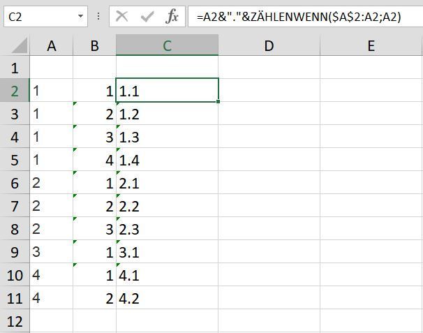
This is the formula in cell C2 in the example:

=A2&"."&COUNTIF($A$2:A2,A2)

This is the formula in cell B2 in the example:

=COUNTIF($A$2:A2,A2)

[#3]

@alexjw94 

Alternatively with Power Query:

[#4]

@alexjw94 alternatively using dynamic array

=LET( in, A2:INDEX(A:A,COUNTA(A:A)),
           counts,DROP(REDUCE(1,SEQUENCE(MAX(in)),LAMBDA(p,q, VSTACK(p,SEQUENCE(SUM(--(in=q)))))),1),
           HSTACK(counts, in&"."&counts))

note that the "in" parameter on line 1 could be entered as a2:a100 instead of auto sizing