Pivot table custom total formula

[vince2397]

Hello,

I have created a pivot table, however I am stuck on 3 calculations, 2 of which are show on the attached screenshot. I am trying to see how I can customize a specific cell calculation.

For example in the highlighted cell with 35.09% (which is calculating an average of above cells), I need it to calculate "Daily GP total($16,895.99)/Daily sales total(39,853.16)" from cells to left which should be 42.39%. I cannot figure out how to customize these certain cells. 

Thank you in advance to anyone that can help.

[#2]

@vince2397 

Adding data to data model you may add DAX measure like

PerCent:=IF(HASONEVALUE(Table[Date]),
            AVERAGE(Table[Percent]),
            SUM(Table[Daily GP])/SUM(Table[Daily sales])
)

[#3]

@Sergei Baklan 

I am sorry, can you give me a bit more direction as to where I would enter/add this? This type of pivot is beyond my area of expertise so I am learning.

Thank you

[#4]

@Sergei Baklan 

I found where you were referencing but receive the following attached error once trying to "Add New Measure"?? Thanks.

Vin

[#5]

@vince2397 

It's bit hard to discuss that with screenshots only.

First, I assume you are on Excel for Windows desktop on version which works with data model (majority of them).

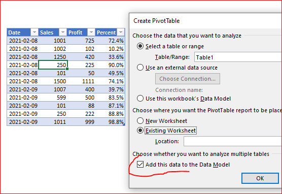
Creating PivotTable check the box as on screenshot to add data to data model

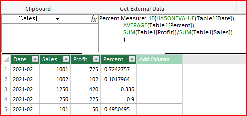
For this sample you may add measure as

Percent Measure:=IF(HASONEVALUE(Table1[Date]),
       AVERAGE(Table1[Percent]),
       SUM(Table1[Profit])/SUM(Table1[Sales])
)

The idea is takes average of profit if only one day selected (e.g. for each row of the PivotTable) and if few days are selected (i.e. for Grand Total) it calculates profit for total numbers, not average of averages. Result is