Pivot Pie Chart for Excel Table - Filtering by dates and staff

[DN4559]

I want to build a pivot cart that will go off this table that contains month to month employee performance grades.

The table headers are months (1/1/2021, 2/1/2021, 3/1/2021, 4/1/2021...)

The table rows are the staff members.

The values for each cell is the staff grade for that month out of 100.

I wanted to create a pie chart that will have a slicer that for the months so I can get a monthly average.  If i wanted a 3 month or 5 month or all time average score. And it will demonstrate with the pie chart.

How can i do that?

Drew

[#2]

Hi @DN4559,

in order to use a Pivot chart, your data needs to be in a "flat" table structure and not in a tabular one.

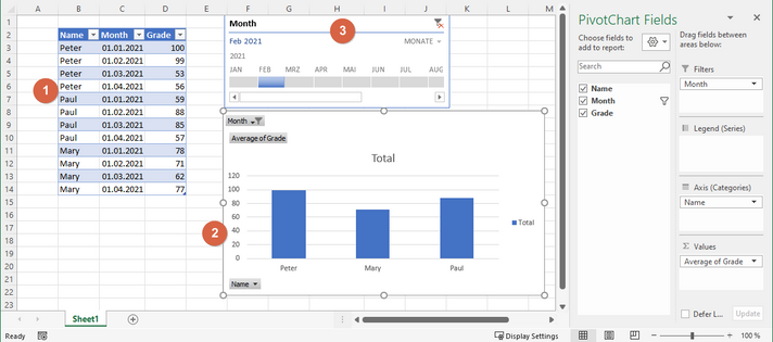
So, the very first thing you need to do is to convert the data from your current structure into something like this:

1. Source data (which is a formatted table)

2. Create the chart: menu "Insert | PivotChart"

3. Insert Timeline: menu "Insert | Timeline"