Partial Miss Match of Vlookup

[daitou]

What I want to do is to find every number of column A in column E and print the relating value in B. 

I find that almost 10% of the number is missed.  I have checked all the possible errors like space or format.

And it is strange that when I find the boxes which are wrong and then re-enter the quoted box, it works as correct. (The video records that phenomenon)

Therefore, I assume that there might be some systematic error with Vlookup function?

In the test file, you can find that some numbers, such as 11.37 and 11.63, are not matched correctly.

Thank you for your help.

Sincerely，

Xinyu

[#2]

@daitou 

Highlight column E, goto the Data tab, click Text to Columns, check that the Delimited radio button is checked and click finish.

[#3]

....I would also suggest that you wrap your formula in an IFERROR function, to avoid the #N/A....then you can calculate the numbers in the result to check that it matches the lookup table.

=IFERROR(VLOOKUP(E2,A$1:B$300,2,FALSE),"") [Enter in cell F2]

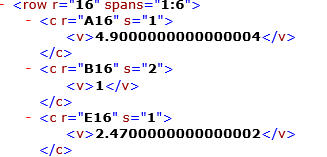
[#4 · Accepted solution]

@daitou 

That is rounding error issue, more about it here EXCEL: RANK, COUNTIF, AND FLOATING POINT ERRORS   If check xml components of your file, quite many numbers looks like

I don't know how did you take them, better to pull numbers correctly. Otherwise use something like

=VLOOKUP(ROUND(E2,15),ROUND(A$1:B$300,15),2,FALSE)

and take into account rounding error could appear in other calculations as well.

[#5]

Thank you very much! It does work ~\(≧▽≦)/~@Charla74 

[#6]

Sure, I will keep it in mind. :ok_hand:

[#7]

The origin data is calculated by another formula that might generate such floating numbers. 

Moreover, I find that =VLOOKUP(ROUND(E2,15),ROUND(A$1:B$300,15),2,FALSE) will get #VALUE! result, however, if I change it into =VLOOKUP(ROUND(E2,15),A$1:B$300,2,FALSE) then it will get the correct results. 

I have downloaded your test file. It shows the correct results at first but when I re-enter the same formula, it turns into #VALUE! error again. Does it mean that my Excel is lack of some plugin?

Anyway, I appreciate your comprehensive explanation. It gives me further insight. ^-^

[#8]

@daitou 

I guess you are on Excel without dynamic array, thus formula shall be used as array one, i.e. entered with Ctrl+Shift+Enter. Anyway, if rounding only lookup value is enough you may use this variant of the formula.

[#9]

@Sergei Baklan Thank you for your help! It seems that I need to update my Excel. O(∩_∩)O

[#10]

@daitou , you are welcome, glad to help