Not able to create a double unary formula on Excel for Mac v16.36

[jayaramv]

Hi, 

I am trying to create a basic SUMPRODUCT formula in Excel for Mac v16.36: 

=SUMPRODUCT(--(B16>{$A3,$A4,$A5,$A6,$A7}),--(B16-{$A3,$A4,$A5,$A6,$A7}),{B$3,B$4-B$3,B$5-B$4,B$6-B$5,B$7-B$6})

I keep getting the "There's a problem with this formula" pop-up. The formula is correct and works perfectly fine in Google Sheets. 

What am I doing wrong? Thank you.

[#2]

@jayaramv 

Excel does not allow range references inside { } - you can only put constants inside the {} syntax.

You need to convert your formula to an Excel-style array formula. If you have Dynamic Array Excel it will automagically be enetered as an array formula, otherwise you need to use Control-Shift-Enter to enter the bformula

[#3]

Thank you. Would you kindly walk me through the steps? I would be very grateful.

[#4]

Can someone please help me convert this formula into an "Excel style array formula"? I do not think I have Dynamic Array Excel.

=SUMPRODUCT(--(B16>{$A3,$A4,$A5,$A6,$A7}),--(B16-{$A3,$A4,$A5,$A6,$A7}),{B$3,B$4-B$3,B$5-B$4,B$6-B$5,B$7-B$6})

[#5]

@jayaramv 

You can check for dynamic array version by seeing if you have the XLOOKUP function.

If B2 contains text or zero try this

=SUMPRODUCT(--(B16<$A3:$A7),--(B16-$A3:$A7),(B$3:B$7-N(B$2:B$6)) )

[#6]

Thank you. Is there supposed to be a N before the B2-B6? I am getting a strange result.

[#7]

Tried your approach. Result is incorrect.

[#8]

@jayaramv 

yes you need the N if B2 contains anything other than zero

What is in B2?

What result do you expect?

What result do you get?

[#9]

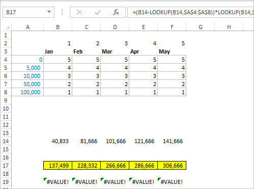
@fastexcel  I've attached a screen shot below. The row in yellow is the set of correct values. Thank you once again for your help. 

[#10]

@jayaramv 

the last part of the formula you have entered is not the same as the formula I used.

 You are using ,--(B$4:B$8)-N(B$3:B$7))

Try ,(B$4:B$8-N(B$3:B$7)))

[#11 · Accepted solution]

@jayaramv 

Thanks for the screenshot: I had a mistake in the formula and also forgot that N() does not return an array. And you don't need the N if B3 is zero.

I think this formula gives you the correct result.

You do not need to array-enter it since SUMPRODUCT always calculates in array fashion. Also you don't actually need the -- in --(B14-$A4:$A8) since there are no True/False to convert to 1s and zeros.

=SUMPRODUCT(--(B14>$A4:$A8),--(B14-$A4:$A8),(B$4:B$8-B$3:B$7) )

[#12]

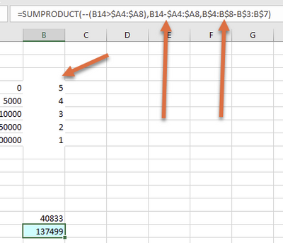
@fastexcel  Worked like a charm. Two observations: 

1. I don't need the 0s in the top row. It works just as well when that row is blank.

2. It doesn't work without the -- 

Screen shots attached. Thank you very much. 

[#13]

@jayaramv 

you need -- on the first sumproduct parameter but not on any of the others.

Yes blank is treated as zero ...

[#14]

@jayaramv 

Just in case, if row 3 is occupied as

it could be

=(B14-LOOKUP(B14,$A$4:$A$8))*LOOKUP(B14,$A$4:$A$8,B4:B8)+SUMPRODUCT(($A$5:$A$8<B14)*($A$5:$A$8-$A$4:$A$7)*B4:B7)

[#15]

"you need -- on the first sumproduct parameter but not on any of the others."

Can you please explain why?

[#16]

@jayaramv 

The first parameter has a > operator which means that the result of the expression will be an array of True or False. SUMPRODUCT will error with True/False so the True/False needs to be converted to numbers, which is done using the --. The other parameters do not have a comparison operator so do not need this.