Noob needs help with function

[Souke555666]

The main job it should do:

Fill column D with value from column CQ but only if value in A = CP

Bonus: if there is no match between A and CP  it should show 0

I have tried VLOOKUP and IF  function and i'm probably not using them correctly.

Tried and failed attempts:

=VLOOKUP($A2;CP:CP;CQ:CQ; [TRUE])

=VLOOKUP($A2;CP:CP;CQ:CQ; [FALSE])

=VLOOKUP(A:A;CP:CP;CQ:CQ; [TRUE])

=VLOOKUP(A:A;CP:CP;CQ:CQ; [FALSE])

=VLOOKUP($A2;CP:CP;CQ:CQ;)

=VLOOKUP(A:A;CP:CP;CQ:CQ;)

=IF($A2=CP:CP;CQ:CQ)

=IF($A2=CP:CP;CQ:CQ; [0])

[#2]

@Souke555666 

=IFERROR(INDEX(CQ:CQ,MATCH(A3,CP:CP,0)),0)

Is this similar to what you are looking for?

[#3]

@OliverScheurich 

Yes this looks like what i'm looking for but i can't seem to test it because i get this annoying ' sign before formula that seem to break it and i don't know how to remove it.
PS. Just deleting it doesn't work since it always shows back up upon finishing the formula.

[#4]

@OliverScheurich 

Previous issue was solved by clearing format

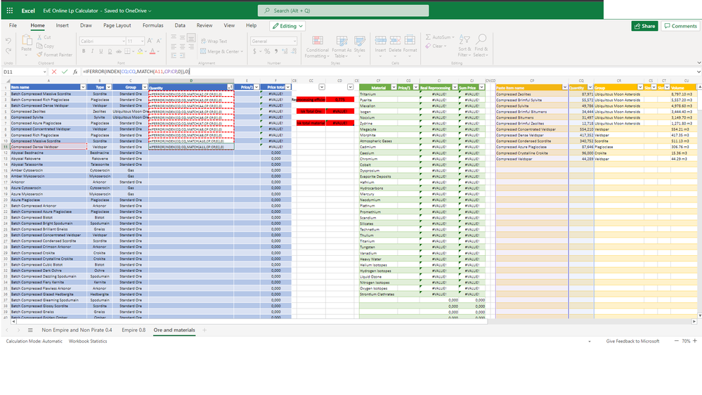
The formula you provided shows up as an error(red boxed)

[#5]

@Souke555666 

Your sample file is too small, i can't see all the details. Can you attach a picture which shows the important data - without sensitive data - in a size similar to the picture of my previous post?

[#6]

@OliverScheurich 

I really do appreciate you trying to help me, thank you mate.

This screenshot should show you all the data involved.

If there is some kind of hidden data that could provide more information let me know how to retrieve it.

[#7]

Bump
Still need help with this.

[#8 · Accepted solution]

@Souke555666 The formulas you mentioned in your initial posting used the semi-colon to separate the arguments. Try replacing the commas in the formula you were given by semi-colons.

Thus, like this:

=IFERROR(INDEX(CQ:CQ;MATCH(A3;CP:CP;0));0)