Nested IF with XLOOKUP

[ADWALLER]

I have a worksheet that I use to create rates for an insurance quote.  I put the person's Age and Annual income in and it tells me how much of the insurance (in dollars) they qualify for (that is just based on their income.  So in column A I have their Age and in column B I have their annual income, and using a formula column C is populated with the amount of coverage they qualify for in dollars.

Then In column D, I want it to calculate the rate for that coverage.  The rate is based on their age and their are 5 age bands (18-49,50-59,60-64,65-69,70+).  So on another worksheet, I have column A which has all the different dollar amounts they could qualify for (From $400 - $2,500 in $100 increments).  Columns B-F are the rates by age band. We know how much they qualify for - it's in column C on the first worksheet A.  So the logic I need to represent in a formula is, look at the amount they qualify for in worksheet 1, column C.  Then go to worksheet 2 and find the row in column A that matches the number in Worksheet 1, column C, the dollar amount qualified for.  Then, depending on the age band they fall into, return the rate that is listed in that age band's column (B-F) that is in the same row as the amount they qualified for.

So figure WKSHT 1 has:

54 years old in column A

$30,000 Annual Income in column B

They qualify for $900/month income replacement - column C

Now on WKSHT 2 we have:

Column A        Column B                 Column C                 Column D

$ Qualified       Rate Ages 18-49        Rate Ages 50-59     Rate Ages (60-69)

$800                $1.50                        $1.75                          $2.00        

$900                $3.00                        $3.25                          $3.50

$1,000             $4.50                        $4.75                          $5.00

$1,100             $6.00                        $6.25                          $6.50

I want the formula to look at the $900 this person qualifies for (from WKSHT 1, Col C) then go to WKSHT 2 and find the $900 in Column A, then go across and return the rate for the persons age - 54 - which should be $3.25.

Here is the concept I was trying working on the =IF functionk:

=IF(D75<50,(D75=XLOOOKUP(J75,'GVDI 773'!C19:C40,'GVDI 773'!D19:D40)),(IF49<D75<59,=XLOOKUP(J75,'GVDI 773'!C19:C40,'GVDI 773'!E19:E40),IF(59<D75<69,=XLOOKUP(J75,'GVDI 773'!C19:C40,'GVDI 773'!F19:F40)))

Any help would be greatly appreciated!

[#2]

@ADWALLER 

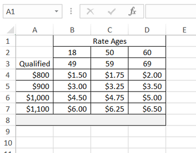
First, I would separate the From/To ages into separate cells. So, I would set up the table like below on Sheet2:

Then, on Sheet1, were A2=54, B2=30000, C2=900, you could enter this formula in D2 to perform your conditional tests and multiply it out (assuming you have office 365):

=SUM((Sheet2!$B$2:$D$2<=A2)*(Sheet2!$B$3:$D$3>=A2)*(Sheet2!$A$4:$A$8=C2)*Sheet2!$B$4:$D$8)

If you don't have office 365, then I would just change "SUM" to "SUMPRODUCT".

=SUMPRODUCT((Sheet2!$B$2:$D$2<=A2)*(Sheet2!$B$3:$D$3>=A2)*(Sheet2!$A$4:$A$8=C2)*Sheet2!$B$4:$D$8)