Nested IF formula in Excel 365

[DanGreene]

Hello, Im having problems getting the right syntax for nexting IF statements.

Basically Im comparing values already placed into cells G5, H5 and I5 to return a value placed into cell E5.

This is the logic Im attempting to create and embed into one cell.

=IF (G5="LOW" and H5="LOW"), then IF (I5="LOW", "T", IF(I5="HIGH", "T", "T"))

=IF (G5="LOW" and H5="HIGH") then IF (I5="LOW", "T", IF(I5=HIGH, "NT", "NT"))

=IF (G5="MODERATE" and H5=LOW) then (I5=LOW, "T", IF(I5="HIGH", "NT", "NT"))

=IF (G5="MODERATE") and H5="HIGH" then (I5="LOW", "OT", IF(I5="HIGH", "T", "OT"))

=IF (G5="HIGH" and H5="LOW") then (I5=LOW, "T", IF(I5=HIGH, "NT", "T"))

=IF (G5="HIGH" and H5="HIGH") then IF (I5="LOW", "OT", IF(I5="HIGH", "T", "OT"))

If anyone can assist, much appreciated...

[#2]

@DanGreene 

Hi! It seems that your final result can be T, NT, OT.

Can you please explain on your words (not formulas) the conditions to apply each one of the results?

Please tag me so that I can come back to this thread.

[#3]

@DanGreene , by the way, expressions like

IF(I5="HIGH", "T", "T")

have no sense, it always returns "T" independently on what do you have in I5

[#4]

@Celia_Alves 

Hello! Thanks for replying.  Yes I am taking  survey results and distilling down the results in 3 categories:

Difficulty, Importance, and Frequency.  I will apply the logic of the excel formula to return a value of T, NT or OT for levels of training needed for my department.

Difficulty has 3 levels, (low, moderate, high), Importance has 2 levels (low, high) and Frequency has 3 levels (low, moderate, high)

The values are assigned from other calculations from survey results <2.5=low, 2.6-3.4=moderate, >=3.5=high.

So in Cell E5, I need to compare values in G5,H5 and I5 using the logic formulas shown to ultimately provide a value of T, OT, or NT .

Hopefully this makes sense!  thank you.

[#5]

@Sergei Baklan

Sergei,

thank you for the reply.  Yes this is true.  In my analysis of data I collected thru employee surveys, I can distill the data given back into either T, OT or NT to populate the cell E5.   Depending on what values are placed into G5, H5, or I5, the outcome may indeed show the value of "T" for both.  These are types of training that my department will need to implement according to those values. 

I see your point though, I could rewrite the formula on those that have the same "training" value to simplify.

[#6]

@DanGreene 

it is still not clear when you want T, NT or NT to appear.

In your words:

- what needs to happen with the values of G5, H5 and I5 to make E5 = T?

- what needs to happen with the values of G5, H5 and I5 to make E5 = NT?

- what needs to happen with the values of G5, H5 and I5 to make E5 = NT?

[#7]

Sergei,

Looking at the example:

=IF (G5="LOW" and H5="LOW"), then IF (I5="LOW", "T", IF(I5="HIGH", "T", "T"))

I have IF(I5="HIGH", "T", "T")) listed this way because there is a third value of "Moderate" that could be in the Cell I5 which should return a value of "T" as well.

thank you

dan

[#8]

@DanGreene 

Dan, sorry, but I didn't catch. The expression in second part

=IF(I5="LOW","T",IF(I5="HIGH","T","T"))

is equal to

= "T"

will it be in I5 "MODERATE", "LOW" or any other value

[#9]

@Celia_Alves

You can think of this has a flow chart type of analysis.  G5, H5 and I5 are prepopulated with HIGH, MODERATE, LOW.

The logic I'm attempting is a flowchart type  layout:

IF G5 LOW AND H5 LOW then Look in cell I5 for value and place the "T", "NT", or OT" in E5

In this case G5 and H5 are LOW and use the following formula to pick which (T, OT, NT) to place in E5 

IF (I5="LOW", "T", IF(I5="HIGH", "T", "T"))

Since LOW is in cell I5 , it results in "T" in E5.

Depending on values in G5 and H5...(Low, Low or Moderate,High or High,High...ect) it changes how the Value in I5 is interpreted to place the T, OT, or NT in E5.  Sometimes it will seem redundant, but the type of training  will cover multiple scenarios.

I hope Im explaining it correctly.

thank you

[#10]

@DanGreene ,

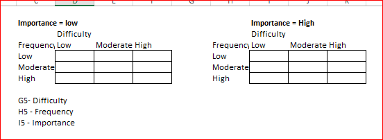
Dan, perhaps it's easier to fill these simple matrices to explain desired result

 (in attached file)

[#11]

@DanGreene, unfortunately, the information you provide is not enough.

You cannot say "Depending on values in G5 and H5...(Low, Low or Moderate,High or High,High...ect) it changes how the Value in I5 is interpreted to place the T, OT, or NT in E5." and expect Excel to know how you are expecting it to interpret the results. The person building the spreadsheet need to teach Excel how to calculate the final result depending on each possible scenario for F5, G5 and H5.

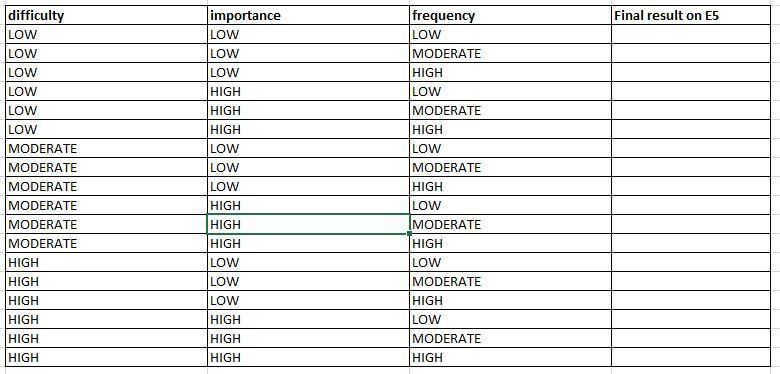
If you follow @Sergei Baklan 's suggestion it will help us find a solution for you. If you prefer, you can also use the structure below to fill in the expected final result for each case.

[#12]

@Sergei Baklan 

Hello,

Attached is my spread sheet.  Hopefully this will help.

Im looking at using 6 logic formulas nested in cell E5 to process the value found I5  to route what formula to use to determine what value  to place into E5.  T, NT, OT.

=IF (G5="LOW" and H5="LOW"), THEN IF (I5="LOW", "T", IF(I5="HIGH", "T", "T")) ELSE

=IF (G5="LOW" and H5="HIGH") THEN IF (I5="LOW", "T", IF(I5=HIGH, "NT", "NT")) ELSE

=IF (G5="MODERATE" and H5=LOW) THEN (I5=LOW, "T", IF(I5="HIGH", "NT", "NT")) ELSE

=IF (G5="MODERATE" and H5="HIGH") THEN (I5="LOW", "OT", IF(I5="HIGH", "T", "OT")) ELSE

=IF (G5="HIGH" and H5="LOW") THEN (I5=LOW, "T", IF(I5=HIGH, "NT", "T")) ELSE

=IF (G5="HIGH" and H5="HIGH") THEN IF (I5="LOW", "OT", IF(I5="HIGH", "T", "OT"))

thank you

[#13 · Accepted solution]

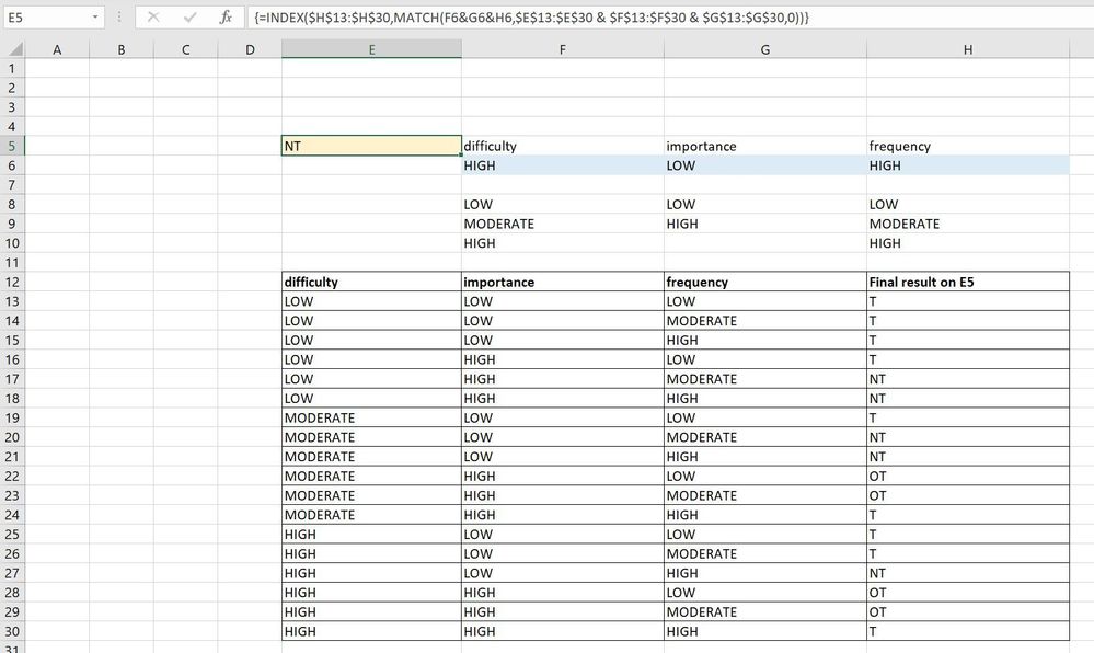
@DanGreene,

please see screenshot and file attached.

The formula that I used is an array formula. To make the formula to work, you need to do CTRL+SHIFT+ENTER after you finish writing it or after you edit it in the formula bar. The formula will get curly brackets at the beginning and ending after you hit those three keys.

Good luck! 

[#14]

Succinctly, what conditions must be fulfilled for the required formula to return each of the possible results? If you cannot answer this question, I am sorry to inform you that you cannot also expect an answer.

[#15]

@Celia_Alves ,

By the way, to simplify the maintenance you may avoid CSE transforming the formula to

=INDEX($H$13:$H$30,MATCH(1,INDEX(($E$13:$E$30=$F6)*($F$13:$F$30=$G6)*($G$13:$G$30=$H6),0),0))

And if the matrix is correct, equivalent nested IF could be

=IF(F6="LOW",
   IF(G6="LOW",
      "T",
      IF(H6="LOW","T","NT")),
   IF(F6="MODERATE",
      IF(G6="LOW",
         IF(H6="LOW","T","NT"),
         IF(H6="HIGH","T","OT")),
      IF(G6="LOW",
         IF(H6="HIGH","NT","T"),
         IF(H6="HIGH","T","OT"))
))

or so

[#16]

@DanGreene 

A different strategy that uses table lookups to determine the training category.

[#17]

@Sergei Baklan 

Sorry, I didn't see this when I posted; I had been away from the computer.

[#18]

That's the type of information we needed. I believe @DanGreene now has a few solutions that can be implemented according to preference. Good luck!

[#19]

That's right, @Sergei Baklan! That's a very nice one too. Thanks!

[#20]

@Celia_Alves , thank you, but nested IF here is only to demonsrate how it looks like. It has no sence in this case - formulas which transform score numbers into text levels are under question. Even if assume they are correct this logic could be changed from time to time. Nested IF with hardcoded conditions is not the a good solution from maintenance point of view.