Need to move informatation from 1 spreadsheet to another spreadsheet and rearrange

[Tinny426]

HI all,
I have tried to work out a formula for what i need, but no success.
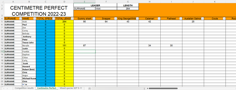
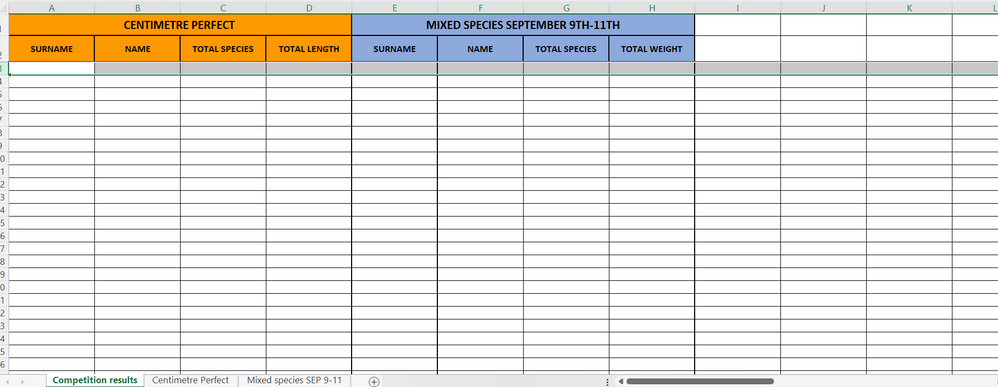
I need to display the first 4 columns of data of the CENTIMETRE PERFECT worksheet (first screenshot) in the first 4 columns of the COMPETITION RESULTS worksheet (second screenshot) in descending order using the values in Column 4.

Can someone give me a formula for what I need? Or is there another solution?

Much appreciated, Richard.

[#2]

Hi @Tinny426 

for sure you could also sort rows that contain formulas. Just select the data table including the headers in row 5 and choose menue "Data | Sort" 

But this is a manual step you have to take. If you really want to automate it (for instance, if some values change), you need to use VBA.

Another option could be the new SORT function that is available in Microsoft 365/Office 365. Here you could for excample create a new worksheet and use SORT with a reference to the original table to get a sorted copy of it.

[#3]

Hello @Martin_Weiss,
Thanks for the reply, its been very helpful. I think the SORT function on another worksheet could do the job. Just need to work this out, as I'm fairly new to the world of Excel.
Cheers Richard.

[#4]

HI all,
I have tried to work out a formula for what i need, but no success.
I need to display the first 4 columns of data of the CENTIMETRE PERFECT worksheet (first screenshot) in the first 4 columns of the COMPETITION RESULTS worksheet (second screenshot) in descending order using the values in Column 4.

Can someone give me a formula for what I need? Or is there another solution?

Much appreciated, Richard.

[#5]

HI all,
I have tried to work out a formula for what i need, but no success.
I need to display the first 4 columns of data of the CENTIMETRE PERFECT worksheet (first screenshot) in the first 4 columns of the COMPETITION RESULTS worksheet (second screenshot) in descending order using the values in Column 4.

Can someone give me a formula for what I need? Or is there another solution?

Much appreciated, Richard.

[#6]

Hi @Tinny426 

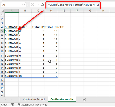
you could use this formula:

=SORT('Centimetre Perfect'!A5:D16,4,1)

Put it in the top left cell of your output range and adjust it to the source range (in my example A5:D16). The formula will spill automatically to all the other cells.

It sorts the table by column number 4 (= second argument)

It sorts the table in descending order (-1 in third argument; ascending would be 1)

Please note that the SORT function is only available in Microsoft 365.

[#7]

Downloading Microsoft 365!

[#8]

Thanks Martin

[#9]

Hi again Martin,
Thanks heaps again for taking the time to help out with my problem. The formula in text was slightly different to the formula outlined in red. But the argument tips you supplied allowed me to make the right changes to get a working formula.
Now i understand how the formula works, i can extend the worksheet as far as i need.
If i ever get to Bavaria, i will look you up and buy you a beer!!
Thanks again Richard.

[#10]

Hello Martin,
I have adjusted the formula above to suit and it works great, but now i want to add another condition!
This is the formula i am using. =SORT('Mixed species SEP 9-11'!A5:D100,3,-1)
In the array above, column C has the letters "S and "J" in random order down the column.
I want to catch only the rows with "S" in column C.
Can this be done? i think i have given enough information above, but i can add screenshots if required.
Cheers Richard.

[#11 · Accepted solution]

Hi Richard,

sure you can, you just need to include the FILTER function. 

=SORT(FILTER('Mixed species SEP 9-11'!A5:D100,'Mixed species SEP 9-11'!C5:C100="S"),3,-1)

Let me know if this works for you.

Cheers,

Martin

[#12]

Hi Martin,
Thanks for your reply, The filter function is just what i was looking for! I wasn't aware of it before.
The formula you gave me works great!:ok_hand:
Cheers Richard.