- Home
- Microsoft 365
- Excel
- Need Help With Sales Inventory Spreadsheet
Need Help With Sales Inventory Spreadsheet
- Subscribe to RSS Feed
- Mark Discussion as New
- Mark Discussion as Read
- Pin this Discussion for Current User
- Bookmark
- Subscribe
- Printer Friendly Page
- Mark as New
- Bookmark
- Subscribe
- Mute
- Subscribe to RSS Feed
- Permalink
- Report Inappropriate Content
Feb 06 2020 01:52 AM
So I'm needing a little bit of help here as I can't seem ti figure this out.
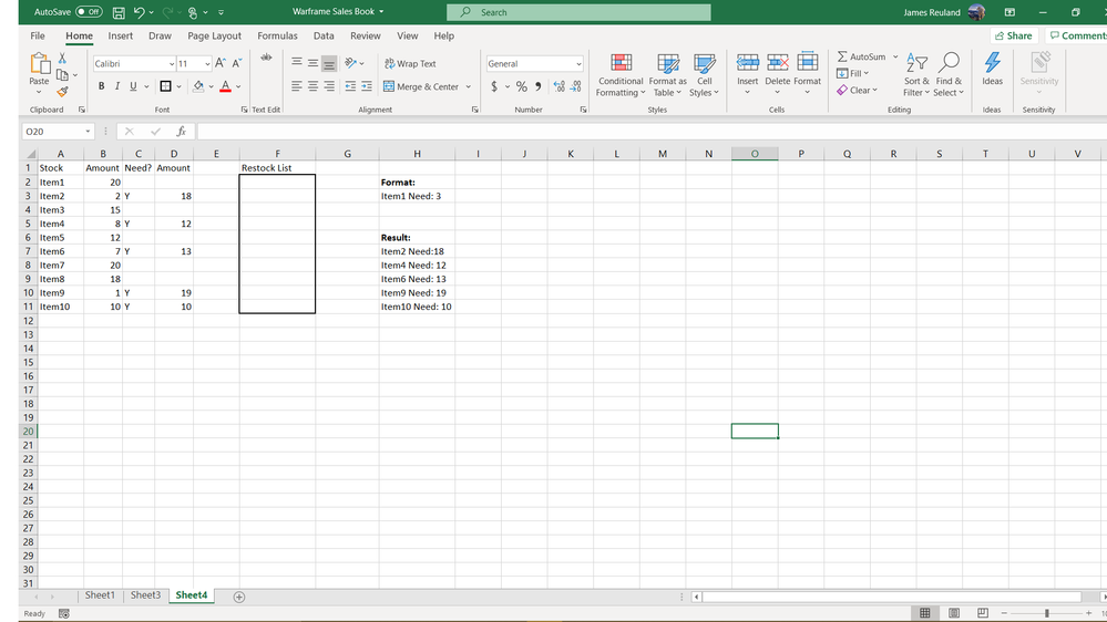
In the picture below is sample model if what I'm trying to do. I'm wanting to set it up so the spreadsheet checks column C for input, in this case the letter Y in a box. If Y is detected, then the information in the corresponding boxes from columns A and D are printed together in the first available box in the Restock list, which in this case is Column F in the formatting I have in H3. If Y is not detected than nothing happens and it just checks the next row and repeats this process for the entire list. The end result in the case of this sample, would look like like in H7-H11 printed in Column F. As normal for it I also need this to active so when I alter the info columns C and D the information in column F automatically clears and is not replaced with a error message.
Now I have tried using a XLOOKUP to do this by putting =XLOOKUP(H1,C2:C11,A2:A11)&" Need: "&XLOOKUP(H1,C2:C11,D2:D11) in the first target box, in this case being F2, with H1 having Y in it as it needs that reference. The problem I face is that It didn't like Y because it wasn't a numerical value so I replaced Y with 1. This fixed that problem however as soon as it found 1 and returned the information, it stopped even though other boxes below also had 1 in it, and I know I can't just renter the formula in the next box as it will just print the same info, and copying the formula shifts all the values down one rather than using the same information.
So I am kind of stumped. I would prefer to use something like Y as it is a clear reference to Yes and then I need it to do this for the entire list.
I have linked the document itself for anyone who would like it.
Any help will be greatly appreciated.
- Labels:
-
Need Help
- Mark as New
- Bookmark
- Subscribe
- Mute
- Subscribe to RSS Feed
- Permalink
- Report Inappropriate Content
Feb 06 2020 02:27 AM
SolutionSince you have access to Excel with XLOOKUP, you may also have the FILTER function. If so, try this:
=FILTER(A2:A11,C2:C11="Y")&" Need: "& FILTER(D2:D11,C2:C11="Y")
- Mark as New
- Bookmark
- Subscribe
- Mute
- Subscribe to RSS Feed
- Permalink
- Report Inappropriate Content
Feb 06 2020 04:39 AM
- Mark as New
- Bookmark
- Subscribe
- Mute
- Subscribe to RSS Feed
- Permalink
- Report Inappropriate Content
Accepted Solutions
- Mark as New
- Bookmark
- Subscribe
- Mute
- Subscribe to RSS Feed
- Permalink
- Report Inappropriate Content
Feb 06 2020 02:27 AM
SolutionSince you have access to Excel with XLOOKUP, you may also have the FILTER function. If so, try this:
=FILTER(A2:A11,C2:C11="Y")&" Need: "& FILTER(D2:D11,C2:C11="Y")
