** Need help with Formula **

[sruk89]

Hi All,

I need help writing a formula based on IF hypotheticals for instance, the value the below field will always change but will always start with one of the following as, me and ma

Switch:

The same applies for these:

Essentially what I'm asking is, IF the start of the the switch begins as, me or ma and IF whether it is RJ45, 1000 BASE-LX etc. and IF it is Copper, Single-Mode etc I want it to automatically select the optic codes as shown below:

Any helps would be super appreciated.

Thanks in advance!

[#2]

@sruk89 

Let's say you have a table with all relevant combinations on a sheet named List in D2:G100.

And let's say that the data in your first three screenshots are in F2, P2 and Q2.

In the cell where you want the formula:

=INDEX(List!$G$2:$G$100, MATCH(1, (List!$D$2:$D$100=F2)*(List!$E$2:$E$100=P2)*(List!$F$2:$F$100=Q2), 0))

If you don't have Microsoft 365 or Office 2021, confirm the formula by pressing Ctrl+Shift+Enter.

Fill down if required.

[#3]

@Hans Vogelaar 

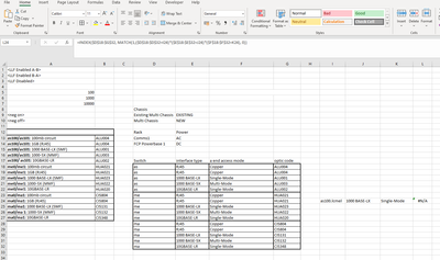
Thanks for your help, i have tried to do the following as mentioned but i cant seem to get it right, please see screenshot below, as mentioned the switch(es) could be a combination of as, me or ma followed by a string of letters after as given I25 but will always start as as, me or ma. the idea is that based on the switch, interface type and access mode, i need it to populate the optic code.

Let me know what im doing wrong :)

Thanks once again :)

[#4 · Accepted solution]

@sruk89

Try

=INDEX($G$18:$G$32, MATCH(1, ($D$18:$D$32=LEFT(I24,2))*($E$18:$E$32=J24)*($F$18:$F$32=K24), 0))

As mentioned before, if you do not have Microsoft 365 or Office 2021, but an older version, confirm the formula by pressing Ctrl+Shift+Enter.

[#5]

Thanks Hans, that worked a treat although I had to remove the a-end access mode but that isn't significant in this case. I truly appreciate your help!