- Home
- Microsoft 365
- Excel
- Re: Need Help Please..... need and IF function or a Formula to assist
Need Help Please..... need and IF function or a Formula to assist
- Subscribe to RSS Feed
- Mark Discussion as New
- Mark Discussion as Read
- Pin this Discussion for Current User
- Bookmark
- Subscribe
- Printer Friendly Page
- Mark as New
- Bookmark
- Subscribe
- Mute
- Subscribe to RSS Feed
- Permalink
- Report Inappropriate Content
Oct 10 2021 05:47 PM
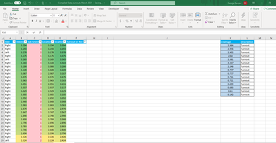
Formulas to assist snippet below
I'm trying to figure out if Values in K column falls in between column D and E?? and have it present, in comumn F, if the turnout values is present between the upper and lower limit.
Column D being the lower limits for that particular chainage and E the Upper limit.
Now I want a formula to help out but I'm no expert in this, been trying to use If and function but doesn't seem right because there are multiple values of the turn out( columnK)??
=IF(AND(D2<$K$2,E2>$K$2),"Turnout","")
but I want to use all the turn out chainages?????
Please Help.
- Labels:
-
Excel
-
Formulas and Functions
- Mark as New
- Bookmark
- Subscribe
- Mute
- Subscribe to RSS Feed
- Permalink
- Report Inappropriate Content
Oct 11 2021 12:19 AM - edited Oct 11 2021 12:24 AM
Solution@ExcelNovice365 -- Since you did not provide a file, I created my own data for illustration purposes. I hope its close enough to your actual data to understand.
I have concluded that you need to re-structure your data such that:
- the LIMITS and CHAINAGES tables are combined into a single table eg "TurnoutDecision", and
- the CHAINAGES values need to be TRANSPOSED and cast as HEADERS
Once the above has been completed, you merely need to
- reference the VALUE(HEADER) in the CHAINAGES portion of the table,
- compare against the LOCATION 1 & 2 with an IF/AND combo statement,
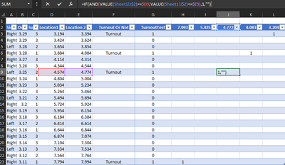
throw a "1" where the VALUE(HEADER) meets the BETWEEN conditions for Location 1, Location 2:
Note we WRAP the HEADER reference in VALUE in order to convert the TEXT format that is forced upon HEADER items into a NUMERAL for SUM purposes. Without the VALUE() function, you'll get nowhere fast.
Next, the TurnoutTest Column performs a SUM on all CHAINAGES by ROW(s):
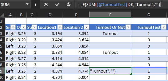
Finally, the "Turnout or Not" column performs an IF on the TurnoutTest value:
Of course, COL F & G are oversimplified here for the purposes of illustration.
I challenge you to combine the "TurnoutTest" & "Turnout Or Not" columns into a single column.
See the attached file.
Lastly, if you need help TRANSPOSING tables data I suggest referencing this: https://stackoverflow.com/questions/60266169/dynamic-arrays-spill-horizontally
/C
- Mark as New
- Bookmark
- Subscribe
- Mute
- Subscribe to RSS Feed
- Permalink
- Report Inappropriate Content
Oct 11 2021 06:54 PM
Accepted Solutions
- Mark as New
- Bookmark
- Subscribe
- Mute
- Subscribe to RSS Feed
- Permalink
- Report Inappropriate Content
Oct 11 2021 12:19 AM - edited Oct 11 2021 12:24 AM
Solution@ExcelNovice365 -- Since you did not provide a file, I created my own data for illustration purposes. I hope its close enough to your actual data to understand.
I have concluded that you need to re-structure your data such that:
- the LIMITS and CHAINAGES tables are combined into a single table eg "TurnoutDecision", and
- the CHAINAGES values need to be TRANSPOSED and cast as HEADERS
Once the above has been completed, you merely need to
- reference the VALUE(HEADER) in the CHAINAGES portion of the table,
- compare against the LOCATION 1 & 2 with an IF/AND combo statement,
throw a "1" where the VALUE(HEADER) meets the BETWEEN conditions for Location 1, Location 2:
Note we WRAP the HEADER reference in VALUE in order to convert the TEXT format that is forced upon HEADER items into a NUMERAL for SUM purposes. Without the VALUE() function, you'll get nowhere fast.
Next, the TurnoutTest Column performs a SUM on all CHAINAGES by ROW(s):
Finally, the "Turnout or Not" column performs an IF on the TurnoutTest value:
Of course, COL F & G are oversimplified here for the purposes of illustration.
I challenge you to combine the "TurnoutTest" & "Turnout Or Not" columns into a single column.
See the attached file.
Lastly, if you need help TRANSPOSING tables data I suggest referencing this: https://stackoverflow.com/questions/60266169/dynamic-arrays-spill-horizontally
/C


