Need formula based on conditions for lower or higher column values

[ramesh98]

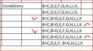
I need help for getting output in Remarks column based on conditions data.

The data is given in attached excel file

[#2]

@ramesh98 

As variant

=IFS(
SUMPRODUCT(--(B3>C3:K3))=9,$H$11,
SUMPRODUCT(--(B3<C3:K3))=9,$H$12,
(B3>C3)*(SUMPRODUCT(--(B3<D3:K3)))=8,$H$13,
(B3<C3)*(SUMPRODUCT(--(B3>D3:K3))=8),$H$14,
(B3>C3)*(SUMPRODUCT(--(B3<D3:K3))=8),$H$15,
(B3<C3)*(SUMPRODUCT(--(B3>D3:K3))=8),$H$16,
(SUMPRODUCT(--(B3>C3:F3))=4)*
(SUMPRODUCT(--(B3<G3:K3))=5),$H$17,
TRUE, "nothing")

In your sample different conditions use same logic

plus some records meet no one. If misprint you may correct the formula as needed.

[#3]

@ramesh98 If you are open to a more graphic representation of the trends, you might want to consider a variety of Sparklines as demonstrated in the attached sheet. In this case, I chose the Winn/Loss type with markers for highest (green) and lowest (red). The "Trend" column in M fairly accurately represents the textual trend descriptions by looking at the placement of the different markers.

Just another way to look at things.

[#4]

@ramesh98 

The conditions in D13 and D15 are the same, and the conditions in D14 and D16 are also the same.

[#5]

Thanks sir, Somewhere there seems to be little mistake from my side. Can you check in attached excel sheet@Sergei Baklan 

[#6]

Thanks sir, at the moment i am looking at answer in text form

[#7]

data corrected, pl check again thanks@Hans Vogelaar 

[#8]

Sir, sorry I have attached data again. There was small error in conditions at D15/D17. Also kindly help resolve in attached sheet itself @Sergei Baklan 

[#9]

@ramesh98 

In L3:

=IFS(B3>MAX(C3:K3),$H$11,B3<MIN(C3:K3),$H$12,AND(B3>C3,B3<MIN(D3:K3)),$H$13,AND(B3<C3,B3>MAX(D3:K3)),$H$14,AND(B3>MAX(C3:D3),B3<MIN(E3:K3)),$H$15,AND(B3<MAX(C3:D3),B3>MIN(E3:K3)),$H$16,AND(B3>MAX(C3:F3),B3<MIN(G3:K3)),$H$17,TRUE,"Other")

Fill down.

[#10]

Sir thanks but still showing name error. Kindly check attached sheet @Hans Vogelaar 

[#11 · Accepted solution]

@ramesh98 Apparently you have an older version of Excel that doesn't have the IFS function.

This version will work in all versions:

=IF(B3>MAX(C3:K3),$H$11,IF(B3<MIN(C3:K3),$H$12,IF(AND(B3>C3,B3<MIN(D3:K3)),$H$13,IF(AND(B3<C3,B3>MAX(D3:K3)),$H$14,IF(AND(B3>MAX(C3:D3),B3<MIN(E3:K3)),$H$15,IF(AND(B3<MAX(C3:D3),B3>MIN(E3:K3)),$H$16,IF(AND(B3>MAX(C3:F3),B3<MIN(G3:K3)),$H$17,"Other")))))))

[#12]

I realize that not all rank 5s or rank 9s are the same, for example. I thought I'd take a different approach to the logic offered and go based on positioning.

=IFNA(VLOOKUP(RANK.AVG(B3,B3:K3),{1,"Long term uptrend intact";2,"Chance of initiation of uptrend";3,"Uptrend initiated";6,"Check support at 20 DEMA";8,"Downtrend initiated";9,"Chance of initiation of downtrend";10,"Long term downtrend intact"},2,0),"Other")

[#13]

Working fine. Thanks a lot sir

[#14]

Working nicely thanks. Will check by adding conditions