Need Automatic Conditional Formatting and the cell next to anything highlighted needs to change

[Aaron_Bennett]

Hello,

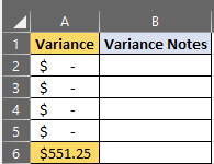
I created an example based on a larger table I have created I need help with having "Column A" automatically having conditional formatting done to highlight the cell if it is not equal to 0 and I want "Column B" to be highlighted as well until a value is entered into it then i wanted it to turn white so that the variance is flagged and the Variance Notes is Flagged until an explanation is entered then it will not be flagged.  I am using Office 365 Pro Plus and have Excel version 1911 (Build 12228.20364)

[#2 · Accepted solution]

@Aaron_Bennett 

Perhaps something like in the attached example. CF rules used are:

=AND(ISNUMBER(A1),A1<>0) in column A:A

and

=AND(ISNUMBER(A1),A1<>0,ISBLANK(B1)) in column B

[#3]

@Riny_van_Eekelen Thank you very much!

[#4]

@Riny_van_Eekelen I have it working and it is a large table that starts with a pivot and then I have IF Statements and Sumif formulas to create four different Actual Vs Budget Comparisons should I create the pivot and copy that information into the table in order to protect all of my formulas so that the pivot doesn't get expanded and overwrite what I have created?

[#5]

@Aaron_Bennett 

Difficult to oversee your exact situation from a screenshot, but if there is a chance that the pivot table (pt) will expand to the right, than I would recommend you not put anything to the right-hand side of the pt. You could consider to put all your formulae and formats on the left-hand side of the pt. Just have the pt starting in e.g. H1 in stead of A1. Alternatively, you can have your pt in a separate sheet and "link" to it, using the GETPIVOTDATA function, in the sheet where you calculate variances and do you all your formatting.

[#6]

How do I use the GETPIVOTDATA Function I have not used it before?

[#7]

@Aaron_Bennett 

May I ask you to read the Excel Help screens first. They are quite extensive and give many examples. If you still feel lost, could you please upload an example of your pt and analysis (with fake data). Then, I can perhaps build a small model that demonstrates what you can achieve with GETPIVOTDATA.

[#8]

@Riny_van_Eekelen Yeah definitely I appreciate your assistance!