- Subscribe to RSS Feed
- Mark Discussion as New
- Mark Discussion as Read
- Pin this Discussion for Current User
- Bookmark
- Subscribe
- Printer Friendly Page
- Mark as New
- Bookmark
- Subscribe
- Mute
- Subscribe to RSS Feed
- Permalink
- Report Inappropriate Content
Mar 24 2022 09:16 AM
Dears,
Kindly need your assist regarding the attached sheet as i need to classify the date to be like the below
| Parameter | 2021 | 2020 | 2019 |
| 0-30 | |||
| 31-60 | |||
| 61-90 | |||
| 91-120 | |||
| 121-150 | |||
| 151-180 | |||
| 181-210 | |||
| 211-240 | |||
| 241-270 | |||
| 271-300 | |||
| 301-330 | |||
| 331-360 | |||
| 360-390 (point of loss) |
Year (C) & dayes of collection (J)
Thanks in advance
- Labels:
-
Excel
- Mark as New
- Bookmark
- Subscribe
- Mute
- Subscribe to RSS Feed
- Permalink
- Report Inappropriate Content
Mar 24 2022 11:38 AM
You'll need the most current version of Excel for this to work (and, I should add, I'm assuming this is actually what you want).
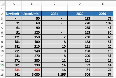
Here's what a count by year and days looks like.
And here's the formula I used.
=LET
(res,
COUNTA(
FILTER('Invoice List'!$A$4:$A$6565,('Invoice List'!$C$4:$C$6565=Aging!C$2)*('Invoice List'!$J$4:$J$6565>=Aging!$A3)*('Invoice List'!$J$4:$J$6565<=Aging!$B3))
),
IF(res=1,0,res)
)
Let us know if that result is what you were seeking. Or if it's totally off base. Or somewhere in between.
- Mark as New
- Bookmark
- Subscribe
- Mute
- Subscribe to RSS Feed
- Permalink
- Report Inappropriate Content
Mar 24 2022 11:44 AM
- Mark as New
- Bookmark
- Subscribe
- Mute
- Subscribe to RSS Feed
- Permalink
- Report Inappropriate Content
Mar 24 2022 12:11 PM
Could i use sum function instead of count for column (F) based on the same criteria
- Mark as New
- Bookmark
- Subscribe
- Mute
- Subscribe to RSS Feed
- Permalink
- Report Inappropriate Content
Mar 24 2022 12:14 PM
- Mark as New
- Bookmark
- Subscribe
- Mute
- Subscribe to RSS Feed
- Permalink
- Report Inappropriate Content
Mar 24 2022 12:59 PM
Could i use sum function instead of count for column (F) based on the same criteria?
- Mark as New
- Bookmark
- Subscribe
- Mute
- Subscribe to RSS Feed
- Permalink
- Report Inappropriate Content
Mar 24 2022 10:51 PM
Explaining how to create a pivot table in two rows is beyond my knowledge.
I'm not a pivot expert, but here's a little guide that I used and started making pivot tables.
First of all, if you look at the inserted file, I have transferred your specifications to a table in the "invoice list" worksheet. The pivot table was then created from this table.
Hope I was able to help you with this information.
I know I don't know anything (Socrates)
- Mark as New
- Bookmark
- Subscribe
- Mute
- Subscribe to RSS Feed
- Permalink
- Report Inappropriate Content
Mar 25 2022 07:02 AM - edited Mar 25 2022 07:06 AM
SolutionCould i use sum function instead of count for column (F) based on the same criteria?
That's the kind of question I'd encourage you to try to answer yourself in the future. All you'd need to do is change the formula. If it works, it works; if it doesn't, see if there was an error in it. One of the best ways to learn whether or not something works is to try it, and tweak it... You definitely don't need to worry about breaking anything.
In this case, I did go ahead and try it. And it worked. Had to make a change at the end too, in the final IF function. It becomes an IFERROR function because in summing when there were no numbers to sum, I got an error message. The IFERROR function handles that. I've highlighted in bold and underlined type the changes. Note: I also created a new tab, entitled "Summing" so that is also new.
=LET(res,SUM(FILTER('Invoice List'!$F$4:$F$6565,('Invoice List'!$C$4:$C$6565=Summing!C$2)*('Invoice List'!$J$4:$J$6565>=Summing!$A3)*('Invoice List'!$J$4:$J$6565<=Summing!$B3))),IFERROR(res,0))
- Mark as New
- Bookmark
- Subscribe
- Mute
- Subscribe to RSS Feed
- Permalink
- Report Inappropriate Content
Mar 25 2022 11:55 AM
But I have a question, please, can you explain the formula of the equation in a simple way so that I can understand it?
- Mark as New
- Bookmark
- Subscribe
- Mute
- Subscribe to RSS Feed
- Permalink
- Report Inappropriate Content
Mar 25 2022 12:38 PM
can you explain the formula of the equation in a simple way so that I can understand it?
Not simply or easily, but I'll try. Here, too, are some excellent resources for you to pursue for more general explanations.
LET function: https://exceljet.net/excel-functions/excel-let-function
FILTER function: https://exceljet.net/excel-functions/excel-filter-function
https://www.youtube.com/watch?v=9I9DtFOVPIg
My formulae use those two functions in particular. FILTER enables you to, well, filter a column or an entire table of data using multiple criteria. In this case, we were filtering a single column, which in the first instance was just the client/customer ID (column A); in the second instance was the size of the outstanding debt (Column F).
Having the "*" sign between sets of criteria operates as if it reads AND. So, first, the criteria
('Invoice List'!$C$4:$C$6565=Summing!C$2)*('Invoice List'!$J$4:$J$6565>=Summing!$A3)*('Invoice List'!$J$4:$J$6565<=Summing!$B3)
are filtering the desired range for either counting or summing based on
- Year (in column c) being the same as whatever is in row 2 of the summary range, which is 2019, 2020 or 2020
- and then the last two criteria determine whether the number of days is greater than or equal to the minimum date, and less than or equal to the greater date of the date ranges you specified.
The COUNTA or SUM functions took the filtered result and counted or summed the rows that came through the criteria in each case, thus resulting in one figure--a count or a sum--for each cell.
[you should experiment with the FILTER function by itself, not nested in COUNTA or SUM, to see what results. Just make sure you leave plenty of rows beneath the formula]
The LET function enables the assigning of the result of the nested COUNTA(FILTER(...)) or SUM(FILTER(....)) to a named variable--I chose "res" as short for "result", and then the closing IF function lets us look at "res" and either just display it or display 0 depending on what its value is.
I used the IF in conjunction with COUNTA because COUNTA always delivers 1 as a result even if the actual number is 0 [because it does show a single row with a text of some kind], so in the case of the COUNTA, the fist time, that closing IF reads IF(res=1,0,res) which just shows 0 if it's getting a 1, but otherwise the full count. In the case of the SUM formula, the final IF is actually an IFERROR because when there's no sum produced it gave an error message.
I know that's a lot to process, especially if, in the first place, you don't understand the various functions. That's why I recommend using the resources linked to above, first of all, and then --even more highly -- I recommend playing with the functions on simpler data arrays until what they're doing makes sense. Play with FILTER by itself, adding criteria and see the results. Then nest FILTER in COUNT or COUNTA or SUM...or any of a number of other functions, and again, see what happens. Same with LET...read the definition in that resource above--or go to YouTube and look there for instructional videos on the LET function. But try it out, use it......just reading about it in something like what I've written above will never fully teach you; we all learn more through doing, and I even emphasize "playing" in the sense of experimenting.
- Mark as New
- Bookmark
- Subscribe
- Mute
- Subscribe to RSS Feed
- Permalink
- Report Inappropriate Content
Mar 25 2022 12:58 PM
Accepted Solutions
- Mark as New
- Bookmark
- Subscribe
- Mute
- Subscribe to RSS Feed
- Permalink
- Report Inappropriate Content
Mar 25 2022 07:02 AM - edited Mar 25 2022 07:06 AM
SolutionCould i use sum function instead of count for column (F) based on the same criteria?
That's the kind of question I'd encourage you to try to answer yourself in the future. All you'd need to do is change the formula. If it works, it works; if it doesn't, see if there was an error in it. One of the best ways to learn whether or not something works is to try it, and tweak it... You definitely don't need to worry about breaking anything.
In this case, I did go ahead and try it. And it worked. Had to make a change at the end too, in the final IF function. It becomes an IFERROR function because in summing when there were no numbers to sum, I got an error message. The IFERROR function handles that. I've highlighted in bold and underlined type the changes. Note: I also created a new tab, entitled "Summing" so that is also new.
=LET(res,SUM(FILTER('Invoice List'!$F$4:$F$6565,('Invoice List'!$C$4:$C$6565=Summing!C$2)*('Invoice List'!$J$4:$J$6565>=Summing!$A3)*('Invoice List'!$J$4:$J$6565<=Summing!$B3))),IFERROR(res,0))

