need a little help

[Tiller610]

So im pretty new and quite stumped.

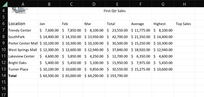
so here in the Top Sales column I need and IF function to determine which two locations had the highest sales. this seems like it should be fairly easy but I've exhausted myself trying to figure it out. 

this is for school and instructions state that the H column needs an IF statement. 

like i can go through each cell and just give it a specific IF function but i feel like that is too easy. i assume there is a better more intuitive way but i cant find it. any help appreciated.

[#2]

Your description is not clear. Do you want the top two locations with the highest sales for each month? If you want to have an output in H column, I assume you are only comparing the data within the same row, which doesn't give you anything.
If you want the top 2 locations of each month, simply use the conditional formatting function under Home - Style, and select Top/Botton rules - more rules. Just configure what you want.

[#3]

sorry brother , my instructions are to use an IF function in column H that will output "Top" in the corresponding h row for the 2 highest earning locations (south park , West spring mall). but i will give the conditional formatting a look. thanks

[#4]

Oh I get what you mean now. Here is the formula
=IF(OR(LARGE($G$7:$G$13,1)=E2,LARGE($G$7:$G$13,2)=E2),"Top","")

BTW the average column doesn't look alright.

[#5]

@Tiller610 

I've made a sample, based on your reference given.

[#6]

@Shiming thank you ill try this, and yea i noticed the average column was off. 

[#7]

wow okay thanks great! thanks!

[#8]

@Tiller610 

I suspect the instructor is looking for something simple:

=IF(OR(G2=MAX($G$2:$G$8),G2=LARGE($G$2:$G$8,2)),"Top","")