Named range created from Excel table used in linked picture

[Zdenek_Moravec]

Dear colleagues,

I have a sheet "Data" with an Excel table full of attributes. On the main sheet, I want to display the first two columns of that table with the possibility of using slicers.

Only way I see is to use "linked picture" (former Camera). It works OK, but new rows are not reflected - the range in linked picture is fixed.

Then I tried the OFFSET function, it works OK for data replicating, but it ignores the filtering using slicers.

FInally I tried to put the OFFSET function to a named range and assign the named range to the linked picture. I get "reference not valid".

How to set a name range created from Excel table in a linked picture?

See attachment with all three attempts.

Of course, if you have other option, how to display filtered data from one sheet in other sheet, let me know.

Thank you very much.

Zdenek Moravec

Cesky Krumlov, Czech Republic

[#2]

@Zdenek_Moravec 

Hi Zdenek,

I'd suggest to add helper column to main table, let name it Visible, 

=(AGGREGATE(3, 5, [@[Project name]])>0)+0

which returns 1 if row is visible and zero otherwise, i.e. if filtered.

For the dashboard we may use

=FILTER(Tab_data[[Project name]:[Manager]],Tab_data[Visible])

which will be synced with main table and shows only visible rows.

[#3]

@Sergei Baklan, thank You for a smart tip. Because I cannot ensure, if all recipients have FILTER function available in our O365, I am afraid, I cannot use it.

In the mean time, I could assign the linked image a named range - the name must be created from INDIRECT function. See solution 5 in the attached example.

It looks like it can work, even the linked picture is not the best solution to reference data from another sheet ...

[#4 · Accepted solution]

@Zdenek_Moravec 

I see. Yes, picture could work but it's not scalable.

One more solution if show visible records wit formula like

=IFERROR(
    INDEX(Tab_data[Project name],
       AGGREGATE(15,6,
          1/(Tab_data[Visible])*
          (ROW(Tab_data[Project name])-ROW(Tab_data[[#Headers],
          [Project name]])),ROW()-ROW($E$38)
      )
   ),
"")

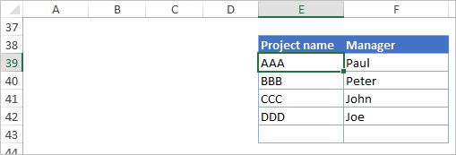
in E39

and drag it down, same for another column. This range will be "filtrable".

[#5]

@Sergei Baklan 

I see now the "scalable" issue - if new row is added,, the picture gets distorted. Then your formula looks like the final solution!

I will try to debug for me. Anyway, can you please explain the AGGREGATE function in human language?

Thank You very much.

Zdenek

[#6]

@Zdenek_Moravec 

Zdenek, AGGREGATE() could do quite many things, in this concrete case with it help we take

Nth (4th parameter ROW() - ROW($E$38) ) smallest (first parameter =15) value from the array (3rd parameter) ignoring all errors (2nd parameter = 6).

Array which we use as 3rd parameter is

1/(Tab_data[Visible])*
(ROW(Tab_data[Project name])-ROW(Tab_data[[#Headers]

First part generates an error for all hided rows in the table (for which Tab_data[VISIBLE] is FALSE or zero, 1/0 generates an error) and second part is sequential numbers of records within the table.

Thus is, for example, there are 4 rows in table and second row is hided, this part returns an array {1,#DIV/0!, 3,4}. Ignoring errors AGGREGATE returns 1 in E39, 3 in E40, 4 in E41 and after that #NUM! error since we are out of source table range.

Wrapping with INDEX we have the value from related record in the table, and wrapping by IFERROR we return empty strings if we are out of range.

[#7]

@Sergei Baklan 

I need more time to understand the aggregate logic, anyway I have put the formulas to my dashboard and it works perfectly!

Thank You very much Sergei, I am glad You are here for us!

Zdenek

[#8]

@Zdenek_Moravec 

Thank you Zdenek, glad to help