Move data up if blank or move to next row and retrieve requested data

[s_psch]

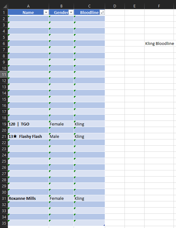
Hi, in the attached sample I have 4 sheets. The main data sheet and three bloodline sheets. Formulas have been added (VLOOKUP, IFERROR, IF) to separate the date on their respective sheets. However, what I want to do is have the data move up if the row above is blank.

or

have a formula check if the correct bloodline is present, if not, move onto the next row and retrieve data that matches the request. 

Office Version: 2021

Thanks in advance.

[#2 · Accepted solution]

I FIRST suggest you use a PivotTable instead and then you add the corresponding filter.

Alternatively (if you really don't want a Pivot Table for some reason), still don't use VLOOKUP etc... and just use FILTER() instead (which according to my MS ref, Excel 2021 should have FILTER and dynamic arrays) so something like:
=INDEX(FILTER(DataTable, DataTable[Bloodline]="Han"), ,{1,9,10})

and if you make $C$1 the filter 'name' so the Header row would be like:

Name    Gender     Han

then the formula could be:

=INDEX(FILTER(DataTable, DataTable[Bloodline]=$C$1), ,{1,9,10})

and quite honestly why even have that last column since it will all be the same?

[#3]

@mtarler, thanks for the reply. Will give it a go and let you know of the outcome.

[#4]

The dynamic filter option actually worked wonders.