max value if criteria match

[vitoaiaco]

Dear all,

I hope you can help me with this.

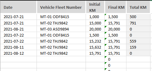
I am trying to generate a spreadsheet that can keep track of fuel consumption. The one responsible for this will enter the information related to mileage once as the vehicles are LEAVING the premises. He will record the mileage again the next time the truck leaves again. The second time he records the mileage, will be the returning mileage for the previous trip, therefore we can record the total mileage for the first trip. In this report I would like to match the truck's fleet number, record the next trip's INITIAL KM and automatically fill in the previous trip's FINAL KM. I hope this makes sense and I hope it's possible. Sample of the sheet is attached, I'm using Excel 2007.

Many Thanks

Vito

[#2]

@vitoaiaco try:

=XLOOKUP(B2,B3:B$99999,C3:C$99999,0,0,1)

[#3]

@mtarler 

Afraid XLOOKUP() doesn't work on Excel 2007.

[#4 · Accepted solution]

@vitoaiaco sry but just notice you said Excel 2007 so use this:

=VLOOKUP(B2,B3:C$99999,2,FALSE)

it does result in #N/A when not found but that is appropriate is it is Not Available yet

[#5]

yea, I notice right after I hit post

[#6]

@vitoaiaco 

As variant

=INDEX($C$2:$C$1000,AGGREGATE(14,6,1/($B$2:$B$1000=$B2)*(ROW($B$2:$B$1000)-ROW($B$1)),1))

gives

[#7]

Thank you both so much, it worked.

Really appreciate your quick responses.

Vito

[#8]

Thank you so much!

[#9]

@mtarler Could I please ask you for another favor?

I have attached the full data input sheet. Apart from tracking mileage, I'm looking also at regularly measuring any reserve left in the fuel tank. Each driver should keep 40 litres of fuel in the tank at all times and this is measured by dipping a level stick into the calibrated tank. Every time a truck goes out, the stick is dipped and we take a record of the level. Would be great if you could help me with a similar formula to match the fleet number with a previous trip and calculating the "float" variance for that particular trip. 

The columns for float and any variance are H and I in the attached file...

Many Thanks

Vito 

[#10]

It sounds like you want the exact same thing but applied to columns H and I, so the same formula could be used but expand the table to include column H and change the 2 to a 5 (to indicate you want the 5th column returned instead of the 2nd):
=VLOOKUP(B2,B3:H$99999,5,FALSE)

[#11]

Yes, but this time I would like to calculate the + or - variance of the two readings. I've tried the following but it doesn't seem to work:
=VLOOKUP(D2,D3:H$99999,5,FALSE)-H5

[#12]

It should work but your refs are a little scrambled (i just opened the sheet and saw some things shifted). Try:
=VLOOKUP(D5,D6:H$99999,5,FALSE)-H5