- Home
- Microsoft 365
- Excel
- Match Dates and TRUE Value for Conditional Formatting
Match Dates and TRUE Value for Conditional Formatting
- Subscribe to RSS Feed
- Mark Discussion as New
- Mark Discussion as Read
- Pin this Discussion for Current User
- Bookmark
- Subscribe
- Printer Friendly Page
- Mark as New
- Bookmark
- Subscribe
- Mute
- Subscribe to RSS Feed
- Permalink
- Report Inappropriate Content
Jul 12 2022 09:14 AM
Hello everyone!
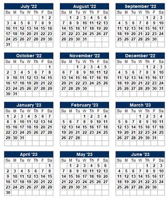
I have a yearly calendar that updates automatically when the start date is changed. This is what the calendar looks like:
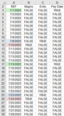
In a separate sheet, I have all of the dates from the calendar with a formula that writes TRUE if the date is in increments of two weeks from a start date. I have conditional formatting set on the dates to change the color when a given column = TRUE.
I am trying to have a similar conditional formatting on the calendar itself to match the REF column's color. Any assistance would be greatly appreciated! Let me know if anymore information is needed.
- Labels:
-
Excel
-
Formulas and Functions
- Mark as New
- Bookmark
- Subscribe
- Mute
- Subscribe to RSS Feed
- Permalink
- Report Inappropriate Content
Jul 21 2022 06:20 AM
SolutionHi all,
Quick update regarding this. I was able to find the solution to what I was looking for:
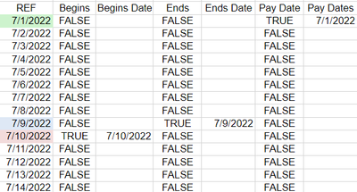
First I isolated the dates for each color I wanted.
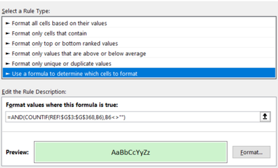
Then used this formula for the conditional formatting and changed the reference column to reflect which dates I wanted highlighted.
I know this was a very niche problem, but in case anyone needs this in the future.
Accepted Solutions
- Mark as New
- Bookmark
- Subscribe
- Mute
- Subscribe to RSS Feed
- Permalink
- Report Inappropriate Content
Jul 21 2022 06:20 AM
SolutionHi all,
Quick update regarding this. I was able to find the solution to what I was looking for:
First I isolated the dates for each color I wanted.
Then used this formula for the conditional formatting and changed the reference column to reflect which dates I wanted highlighted.
I know this was a very niche problem, but in case anyone needs this in the future.


