Manual calculation formula for Duration

[Ravi_RV]

Can any one explain the formula for duration.

[#2]

@Ravi_RV 

Please provide more detailed information.

[#3]

@Ravi_RV 

Presumably, you are asking about the Excel DURATION function (click here).

As usual, the Excel help page is woefully inadequate.

According to the help page, Excel DURATION calculates the Macaulay duration (click here).

If you are unfamiliar with the financial concept, be sure to also read the beginning of that wiki page (click here).

FWIW, you might also look at the implementation presented in a wallstreetmojo.com article (click here).  See ERRATA, posted later.

I struggle with bond concepts.  So I will not attempt to vet that information.

But looking briefly at the math formulas in the wiki page, it is obvious that, at the very least, they need to be modified to account for the various "day count" methods.

(Most presentations assume whole-year maturity and coupon schedules, so the "day count" method might not matter much -- except for accounting for leap years perhaps, but unlikely.)

In the "good old days", we might expect to find a description of the Excel implementation in the help page (albeit not always accurate) and/or a "KB" article.

I have not (yet) found anything like that from MSFT.

[#4]

@Ravi_RV 

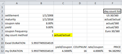
The following demonstrates a "manual" implementation of Excel DURATION when the maturity date is an annual anniversary of the settlement date (i.e. same month and day).  See the attached Excel file for details.

Formulas:

B10: =DURATION(B3,B4,B5,B6,B7,B8)

B12: =100*(SUMPRODUCT(ROW($A$1:INDEX(A:A,D12)),
          PV(C12,ROW($A$1:INDEX(A:A,D12)),0,-E12))

          + D12*PV(C12,D12,0,-1)) / B7 / F12

C12: =B6/B7

D12: =COUPNUM(B3,B4,B7,B8)

E12: =B5/B7

F12: =PRICE(B3,B4,B5,B6,100,B7,B8)

The formula in B12 is based on the description in the wiki page (click here).

ROW($A$1:INDEX(A:A,D12) produces a row array of integers {1; 2; ... ; D12},  stylistically.  It can be replaced with SEQUENCE(D12,1) in Office 365 and later versions of Excel.

t[i] (time in years) is calculated by ROW($A$1:INDEX(A:A,D12) / B7).  The factor 1/B7 is removed from SUMPRODUCT algebraically.

PV[i] (present value of each coupon payment per 100) is calculated by

PV(C12,ROW($A$1:INDEX(A:A,D12)),0,-E12).

t[n]*FV (present value of the face value payment per 100) is calculated by

D12*PV(C12,D12,0,-1).

TBD:  An "adjustment" in my implementation is needed to handle the case when the maturity date is not an annual anniversary of the settlement date.

-----

An important point to note is:  for Excel DURATION, yield (B6) is treated as a simple ("nominal") rate, whereas the wiki page suggests that it should be treated as a compound ("effective") rate.

I cannot say, with impunity, which is correct.  But the Excel DURATION calculation agrees with one online calculator (click here), which is not authoritative.

ERRATA:  My previous posting cited one description of a "manual" Excel calculation (click here).  I removed that citation because it treats yield as a compound rate, unlike Excel DURATION.

[#5]

I wrote:

B12: =100*(SUMPRODUCT(ROW($A$1:INDEX(A:A,D12)),
          PV(C12,ROW($A$1:INDEX(A:A,D12)),0,-E12))

          + D12*PV(C12,D12,0,-1)) / B7 / F12

C12: =B6/B7

D12: =COUPNUM(B3,B4,B7,B8)

E12: =B5/B7

F12: =PRICE(B3,B4,B5,B6,100,B7,B8)

-----

If you want a formula for DURATION that you can implement in other languages, you might prefer the following.

B12: =100*(SUM(i*E12/(1+C12)^i, for i=1 to D12)
          + D12/(1+C12)^D12) / B7 / F12

C12: =B6/B7

D12: =(YEAR(B4)-YEAR(B3))*B7

E12: =B5/B7

F12: =100*(SUM(E12/(1+C12)^i, for i=1 to D12) + 1/(1+C12)^D12)

Obviously, the formulas in B12 and F12 are not bona fide Excel formulas.

The formula in D12 relies on the simplifying assumption that the maturity date is an annual anniversary of the settlement date (i.e. same month and day).