Mailing list from Power Pivot

[bartvana]

I have 3 tables:

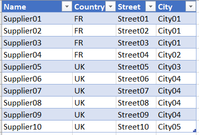
• a dimension table with suppliers,
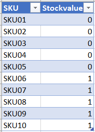
• a dimension table with SKU's,
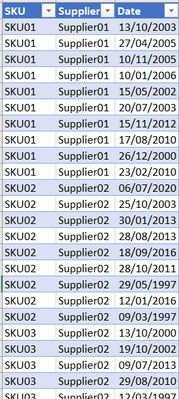
• a fact table of purchase orders.

(See simplified data below and in attached workbook).

tSuppliers:

tSKUs:

tPOs:

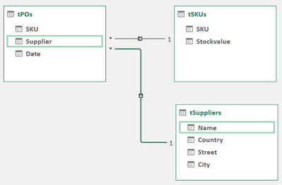
I have added these to a Power Pivot model.

I now want to have a mailing list of the suppliers that:

• have a purchase order between 2015 and 2020
• concerning only SKU's that have stockvalue = 1

The mailing list needs to have the same columns as my Suppliers table (it's actually a filtered list of the Suppliers table).

I can do this in Power Query or with XLOOKUP's and formula's, but my question is: is it possible to generate such a list using Power Pivot only?

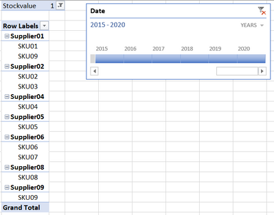
I got this far:

but I have two problems:

1. The mailing info is missing of course (Country, Street, City)
2. The Stockvalue filter isn't working. Stockvalue is filtered = 1, but eg. SKU01 has Stockvalue = 0 and still it is listed.

So my questions are:

1. Why is the stockvalue filter not working?
2. If such a mailing list can be generated with a Power Pivot Pivot table, how?
3. If this is impossible in Power Pivot, what would your most efficient general approach be to creating such a mailing list?

(My real data and filter requirements are obviously a bit more complex, so I'm interested rather in methods and strategies, than a quick solution for the simplified sample data).

Many thanks in advance!

[#2]

@bartvana Perhaps the attached file helps.

[#3]

@Riny_van_Eekelen So actually the Stockvalue filter was already working, right? I misinterpreted the data, I see now.

If I'm correct, you tweaked the PivotTable with the Design options? Or did you do something else too?

[#4]

@bartvana Didn't tweak much more than choosing a tabular layout. Other than that, I also changed the selection of fields (Row, Column and Value) as you can see in the pivot table fields window.

[#5 · Accepted solution]

@bartvana 

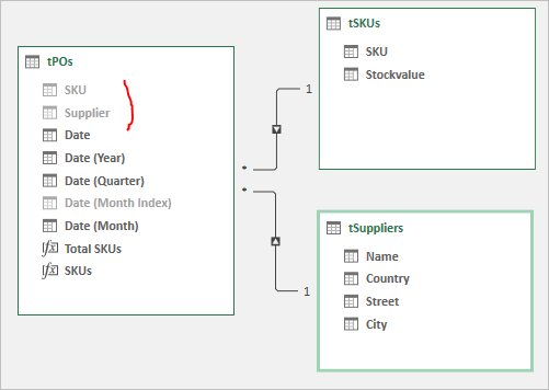
As a comment, that's a best practice to hide fields on "many" side of relationship and don't use them in reports.

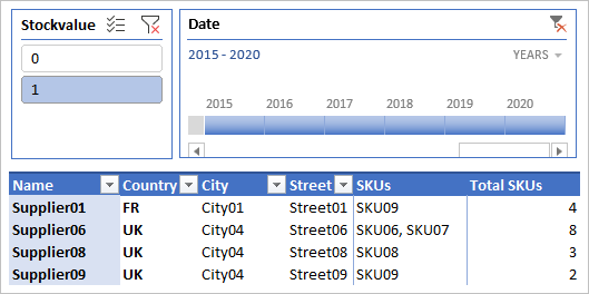
Slightly modified @Riny_van_Eekelen  solution, you may use measures

Total SKUs:=CALCULATE( COUNTROWS( tPOs ), CROSSFILTER( tSKUs[SKU], tPOs[SKU], Both ) )

SKUs:=CALCULATE( CONCATENATEX(tSKUs, tSKUs[SKU], ", "), CROSSFILTER( tSKUs[SKU], tPOs[SKU], Both ) )

to have PivotTable in bit different form

[#6]

@Sergei Baklan Thank you for the tips.

Thank you both for your help!

I'm just not sure which answer to mark as best response now :)

[#7]

@bartvana A like will do. Haha!

[#8]

@bartvana 

Actually Best responses and likes are only help to promote this resource (TechCommunity) on the web. More of them more visible the resource. Just SEO stuff.

From personal point of view that doesn't matter, at least for me. Anyway, thank you for the feedback.