Lookup/bring in values from data array into table

[Jpalaci1]

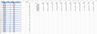
I want to take the data from an array and lookup based on the ID #, current month, and correct year but not sure how to get there.

I put the answer of how it should be to the right of the table but not sure how to get it from the data on the right to the table on the left.

 

[#2 · Accepted solution]

@Jpalaci1 

There are many variations that can be used depending both upon personal preferences and Excel version.  Since I develop for Excel 365, I would go for INDEX and XMATCH, though XLOOKUPS would also be possible.  A common trick for matching two rows/columns is to concatenate them.  In the present case, the year and month can be combined more naturally as an Excel date serial value.

= LET(
  date,    DATE([@Year], [@Month], 1),
  dateHdr, DATE(year, month, 1),
  rowNum,  XMATCH([@ID],ID),
  colNum,  XMATCH(date, dateHdr),
  INDEX(Value, rowNum, colNum) )

[#3]

Thank you! That really helped. Thank you for showing me the names ranges. I was aware of them but never really used them. Definitely use way more.

[#4]

@Jpalaci1 

Thanks for the feedback.  I haven't used a cell reference since 2015, but that is a matter of personal taste!  Something else you might like to try is to copy the formula somewhere outside the confines of the table ([@Year] should now read Table1[@Year]) and the result could be a single value or an error depending on the row in which you place the formula.

Now remove the '@' so that entire ranges are referenced; you should get the result array as a spilt range.